Choosing, carrying out and concluding a statistical test

Choosing the test

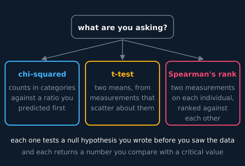
Three tests cover almost everything an A-level investigation produces, and choosing between them is a question about the shape of your data rather than about the biology.

Describe the drawing

A single box at the top asking what kind of question is being asked, with three arrows fanning out to three cards below. Each card names one test and lists in three short lines the kind of data it takes: counts in categories against a predicted ratio, two means from scattered measurements, and two different quantities measured on each individual, each ranked on its own.

Two conditions are worth checking first. Chi-squared needs raw counts, never percentages, and every expected value should be at least 5; combining categories or collecting more data is the fix when they are not. The t-test assumes measurements that are continuous and roughly normally distributed, which lengths, masses and volumes usually are and counts of individuals usually are not, and it assumes the two samples are about equally spread. That last condition is stated less often than the others, and the A-level formula depends on it, as the next section shows.

A normal distribution is symmetrical and bell-shaped: the mean, median and mode coincide, and about 95% of values lie within two standard deviations of the mean. The heights of plants of one species usually look like this. A non-normal distribution is lopsided, as the number of parasites per host is. Most hosts carry few or none and a handful carry a great many, so the mean sits well above the median. A test that assumes normality should not be used on it.

One distinction decides the choice here: 'two measurements per individual' does not automatically mean Spearman. Spearman asks whether two different quantities are associated, moisture against species count. Measuring the same quantity twice on each individual, before and after a treatment, is a difference question, and the tool built for it is the paired t-test. OCR A provides its formula and can set it; the other specifications do not name it. On any board, before-and-after data call for the differences rather than a correlation: work out each individual's difference and apply the formula below to those differences.

t = d̄√n ÷ s_dd̄ is the mean of the n differences and s_d their standard deviation; degrees of freedom = n − 1

All three then work the same way. Calculate a number from your data, work out the degrees of freedom, look up the critical value at p = 0.05, and compare. For all three, a calculated value at or above the critical value means reject the null hypothesis. Spearman's is the one to watch, because its value runs from −1 to +1 and it is the size you compare: a correlation of −0.87 is exactly as significant as one of +0.87 and points the other way.

Describe the drawing

Two number lines, one above the other. On the first the critical value of 7.81 is marked with an upright tick and everything beyond it is shaded as the rejection region; the calculated chi-squared of 3.87 sits well short of the tick, so the null hypothesis is not rejected. On the second the critical value is 2.10 and the calculated t of 2.96 sits inside the shaded region beyond it, so the null hypothesis is rejected. The two thresholds are at different places because each test has its own.

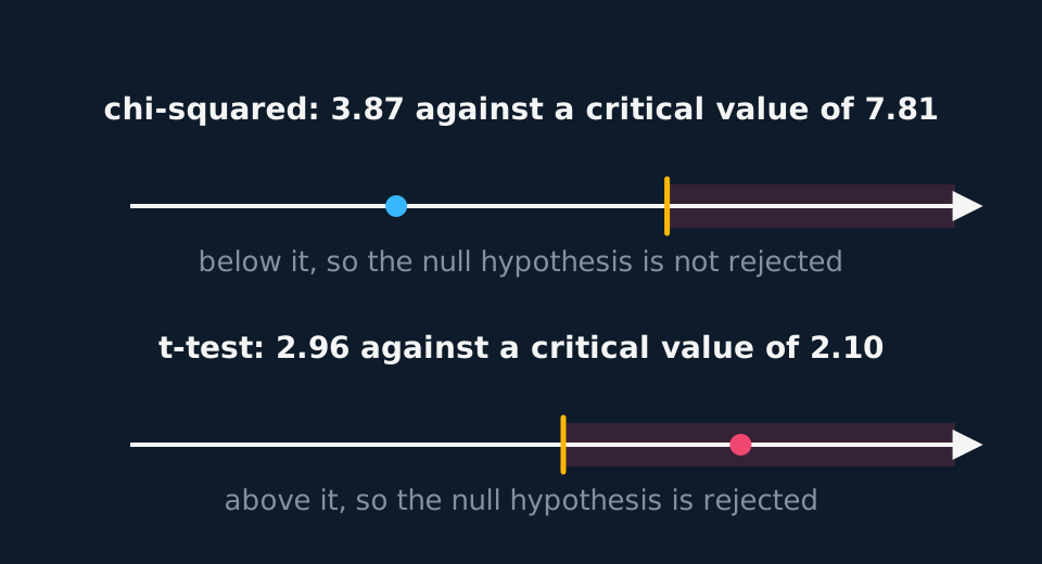
That threshold is not a number to learn. Chi-squared with 3 degrees of freedom needs 7.81, a t-test with 18 needs 2.10, and Spearman with ten pairs needs 0.648; all three come from a table the paper supplies, read against the conditions of your own investigation. What carries from one test to the next is the comparison, not the number.

The three tests, worked

The numbers below are constructed, chosen so the arithmetic stays readable. The sequence of steps is identical every time.

chi-squared = Σ [ (O − E)² ÷ E ]O is the observed count, E the expected count, and the sum runs over every category

Use the t-test formula and degrees-of-freedom rule supplied by the examination paper or data sheet. Cambridge International 9700 supplies a two-sample formula with n₁ + n₂ − 2 degrees of freedom for the data it sets. If the samples have very different spreads, identify this as a limitation of applying that model.

t = (x̄₁ − x̄₂) ÷ √( s₁²/n₁ + s₂²/n₂ )take the difference between the means as a positive number; degrees of freedom = n₁ + n₂ − 2, on samples whose standard deviations are of similar size

Beyond A level the two-sample case is handled by two named tests. Welch's t-test uses the denominator above but calculates its degrees of freedom from the two variances rather than from n₁ + n₂ − 2. The pooled Student t-test, to which n₁ + n₂ − 2 properly belongs, combines the two spreads into a single pooled estimate first. The A-level formula takes the denominator from one and the degrees of freedom from the other, which is a simplification that holds where the samples have similar spreads.

r_s = 1 − [ 6 Σd² ÷ n(n² − 1) ]d is the difference between the two ranks of one individual, and n is the number of individuals, not the number of measurements

Ranking has one detail that gets tested: equal readings take the mean of the positions they occupy. Values of 3, 7, 7 and 9 rank as 1, 2.5, 2.5 and 4, because the two sevens would have held positions 2 and 3, and the next value still takes position 4.

There is a fourth test on the Cambridge International list, and it is Spearman's partner. Pearson's linear correlation coefficient, written r, answers the same question about two quantities measured on the same individuals, and it also comes out between −1 and +1 with the sign giving the direction. They differ in what they work on. Spearman throws the measurements away and keeps their order; Pearson uses the measurements themselves, and asks how well a straight line fits them.

r = Σ[(x − x̄)(y − ȳ)] ÷ √( Σ(x − x̄)² × Σ(y − ȳ)² )x and y are the two measurements on one individual and x̄ and ȳ are their means; the critical value is read for n − 2 degrees of freedom, where n is the number of pairs

That difference decides which one to use. Plot the scatter graph first, before choosing anything. Use Pearson's r when both variables are continuous measurements, when each is roughly normally distributed, and when the scatter looks like a straight line with the points spread evenly along it. Use Spearman's rank when any of those fails. That covers data that are ranks or scores, an obviously skewed distribution, and a small sample. It also covers outliers a straight line would be dragged about by, and a scatter that rises steadily but along a curve instead of a line.

Describe the drawing

Three scatter graphs side by side, each holding forty points and each with two coefficients printed beneath it. In the first the points lie along a rising straight line with a little scatter, and Pearson's and Spearman's coefficients agree at about zero point nine five. In the second the points rise along a curve that flattens at the left and steepens sharply at the right, and Spearman's coefficient is exactly one while Pearson's is far below it. The third repeats the first with a single point moved far above the others, drawn in coral; Spearman's coefficient has barely moved while Pearson's has roughly halved.

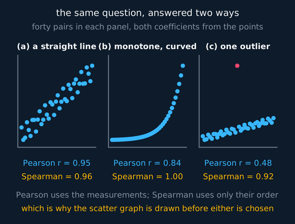
Pearson is preferred where it is allowed because it uses more of the information. It knows how far apart the readings are and not merely which came first. So with data that meet its conditions it detects a real association from a smaller sample. Spearman assumes almost nothing, so it is the test A-level fieldwork usually needs. The two names for that distinction are examinable. A test that assumes a distribution is parametric (on these specifications, Pearson's r and the t-test), and a test that does not is non-parametric (Spearman's rank and chi-squared).

Two warnings apply to both. A coefficient near zero means no linear association for Pearson and no consistent rise or fall for Spearman. Neither of those means no relationship: a variable that rises and then falls again can give an r of almost nothing while being strongly related to the other. And a significant correlation of either kind is still a correlation. The conclusion says that the two quantities are associated, not that one causes the other.

Writing the conclusion

Report four elements in the conclusion: the calculated and critical values, the probability level and degrees of freedom or sample size used, the decision about the null hypothesis, and the biological interpretation.

If the calculated value does not reach the critical value, state that the null hypothesis is not rejected. This means that the data do not provide sufficient evidence against it; it does not show that the null hypothesis is true. The alternative wording, that the null hypothesis is accepted, is widely used and accepted at A level, but it asserts more than the test supports, since a small sample can easily miss a real but small difference. In an evaluation, 'a larger sample might have detected a difference this one could not' is the clause to add.

Reserve 'significant' for the outcome of a test. In ordinary use it means important; here it means the calculated value reached or exceeded the critical value at the stated probability. A difference is not significant unless a test says so, and a significant difference is not necessarily a large one.