Biology › Scientific method and quantitative biology › Averages, spread and the null hypothesis
Averages, spread and the null hypothesis
Biological material varies, so a difference between two means is never self-evidently a difference. Three things have to be settled before any test can be run: which average stands in for the readings, how widely they are spread, and what exactly the test is going to try to disprove.
In two parts Statistics for biologists: spread, error bars and the three tests, part 1 of 2. Part 2 is Choosing, carrying out and concluding a statistical test.
Before this Calculating a mean · Drawing and reading a scatter graph
COMMON MISCONCEPTION
If the error bars on two means do not overlap, the difference between them is significant.
Interpret error bars only after identifying whether they show standard deviation, standard error or a confidence interval. Their overlap does not by itself establish statistical significance; use the appropriate statistical test.
What you should be able to do
- Choose between a mean, a median and a mode for a given set of biological data, and say why.
- Calculate a standard deviation and explain what it shows that a range does not.
- Interpret error bars, including what non-overlapping bars do and do not prove.
- State a null hypothesis naming both variables and the populations.
Mean, median, and the reason a range is not enough
The first job of a statistic is to stand in for a whole set of readings, and which one you choose depends on what those readings look like.
- Mean
- The total divided by the number of readings. Uses every value, and is what almost every biological calculation wants.
- Median
- The middle value when the readings are put in order. Unmoved by a single extreme value, which is why it is used for skewed data such as incomes, reaction times or the number of parasites per host.
- Mode
- The most common value. The only one of the three that works for categories such as blood group or flower colour.
One number is never enough, because two sets of readings with the same mean can be entirely different sets. What goes alongside it is a measure of spread, and the obvious candidate, the range, turns out to be a poor one.
Describe the drawing
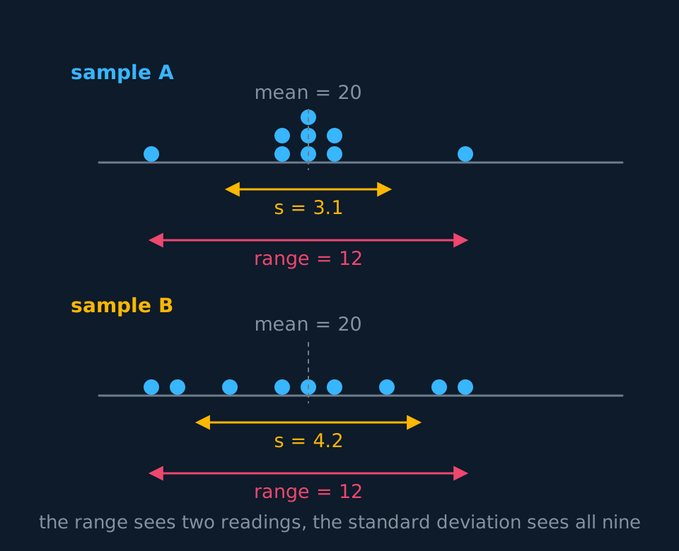
Two dot plots one above the other on identical horizontal scales. The upper set piles most of its dots on top of one another near the middle with one dot far out on each side; the lower set spreads its dots evenly across the same width. Below each plot a short amber bar marks one standard deviation either side of the mean and a longer coral bar marks the full range, and the two coral bars are the same length while the amber ones are not.
The range uses two numbers and discards the rest, so it cannot tell readings that cluster tightly with two outliers from readings spread evenly. It also gets worse as you collect more data, since more readings means a better chance of catching an extreme one, and a statistic that depends on how long you spent measuring is not describing the organism. The standard deviation fixes both problems: it is roughly the typical distance of a reading from the mean, and every reading contributes to it.
s = √[ Σ(x − x̄)² ÷ (n − 1) ]sum the squared deviations from the mean, divide by one less than the number of readings, take the square root
The n − 1 is not a typo. The sample's own mean is being used to measure the sample's spread, which makes the deviations slightly too small, and dividing by n − 1 corrects for it. A version with n on the bottom is also a real formula, and it belongs to a complete population, where the mean is the population's own and there is nothing to correct. That is why a calculator offers two standard deviation keys, usually labelled sample and population, or s and σ. Biological readings are a sample drawn from something larger, so n − 1 is the one to reach for, and it is the form written on the formula sheets that print a standard deviation for biology. If a question gives you a formula, use that one.
A standard deviation from nine readings
Sample A consists of the nine readings 14, 19, 19, 20, 20, 20, 21, 21 and 26. Sample B consists of 14, 15, 17, 19, 20, 21, 23, 25 and 26. Both sets are idealised, chosen so that the arithmetic stays visible. Calculate the mean and standard deviation of each and comment.
Show the working
Both totals are 180, so both means are 180 ÷ 9 = 20; both medians are the fifth value in order, which is 20; both ranges are 26 − 14 = 12. On every statistic so far the samples are identical.
For sample A the deviations from the mean are −6, −1, −1, 0, 0, 0, +1, +1 and +6, whose squares total 76. Then 76 ÷ 8 = 9.5, and √9.5 = 3.08.
For sample B the deviations are −6, −5, −3, −1, 0, +1, +3, +5 and +6, whose squares total 142. Then 142 ÷ 8 = 17.75, and √17.75 = 4.21.
Sample B is about a third more variable than sample A, and nothing except the standard deviation said so. Squaring does the work: it makes every deviation positive so they cannot cancel, and it weights a reading six from the mean thirty-six times as heavily as one a single unit away.
Error bars, and the claim they do not support
An error bar shows how much the readings behind a mean varied, or how precisely the mean is known. It turns a column that looks like a fact into a column with a width, which is the truthful way to draw a biological measurement.
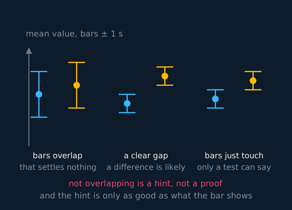
The first question about any error bar is what it was drawn from, because three things are commonly used and they mean different things:
| Bar | What it shows | What happens as the sample grows |
|---|---|---|
| ± 1 standard deviation | How much the individual readings vary | Stays about the same: it is a property of the organism |
| ± 1 standard error (SE = s ÷ √n) | How precisely the mean has been estimated | Shrinks, roughly as one over the square root of n |
| 95% confidence interval | Mean ± 2 SE; intervals drawn this way contain the true mean in about 95 samples in 100 | Shrinks, and is roughly twice the standard error for a decent sample |
For sample A in the example above, s = 3.08 and n = 9, so SE = 3.08 ÷ √9 = 1.03, and the 95% confidence interval is 20 ± 2.1, from 17.9 to 22.1.
The table is why the overlap rule fails. Standard-deviation bars describe variation between organisms and barely narrow however many you measure, so two genuinely different means can easily have overlapping SD bars. Standard-error bars describe how well you know the mean and shrink with sample size, so with a large enough sample almost any two means separate. The same data drawn two ways gives opposite impressions, and neither drawing is a test.
Bar overlap alone does not establish statistical significance, so the sentence to write is 'the error bars do not overlap, which suggests a difference; a t-test is needed to establish whether it is significant.'
Error bars also describe what varied. If the bars on a graph of enzyme activity are long at 50 °C and short at 20 °C, that is a finding: the reaction has become less repeatable near the denaturation threshold, and saying so is better biology than describing the means alone.
The null hypothesis, and what p = 0.05 actually says
Every statistical test starts from a null hypothesis: a specific statement that there is no effect. It is written before the data are looked at, and the test's one job is to ask whether the data are awkward for it.
- Null hypothesis
- A statement that there is no significant difference, no significant association or no significant correlation between the variables, and that any difference observed is due to chance.
- Significance level
- The probability threshold, conventionally 0.05, below which the null hypothesis is rejected.
- Degrees of freedom
- A number, worked out from the number of categories for chi-squared or from the sample sizes for a t-test, that decides which critical value you read from the table.
Name both variables and the populations in the null hypothesis. The form of the sentence is the same whichever of the three tests below follows it. Next topic: choosing and concluding a statistical test.
| Test | A null hypothesis stated in full |
|---|---|
| Chi-squared | There is no significant difference between the observed numbers of offspring in each phenotype and the numbers expected from a 9:3:3:1 ratio. |
| t-test | There is no significant difference between the mean shell length of limpets on the sheltered shore and the mean shell length of limpets on the exposed shore. |
| Spearman's rank | There is no significant correlation between soil moisture content and the number of plant species per quadrat. |
A p-value is the probability of obtaining a result at least as extreme as the one observed, if the null hypothesis were true. It is often shortened to 'the probability that the difference is due to chance', which is accepted at A level, but the full statement matters because the short form supports two false conclusions.
It does not say there is a 95% probability the effect is real. The p-value is calculated assuming the null hypothesis is true, so it cannot then say how likely that assumption was. And it says nothing about the size of the effect: half a millimetre between two mean shell lengths will come out significant if you measure enough limpets, because significance depends on sample size as much as on the difference. Significant means unlikely to be this big by chance alone, and the sentence after a significant result should always say how big the difference was as well as that it was there.
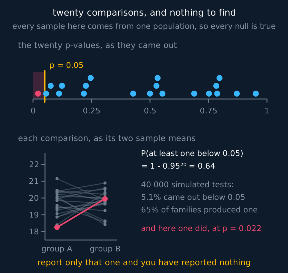
The 0.05 is a convention and it sets what you are willing to risk: one time in twenty you will reject a true null hypothesis and announce an effect that is not there. That is the cost of the test, and it is why a study that runs twenty comparisons and reports the one that came out significant has reported nothing.
Describe the drawing
Two drawings of one set of twenty comparisons. Along the top, the twenty p-values are plotted as dots on an axis running from zero to one, with the region below nought point nought five shaded and marked by an upright amber line; one dot falls inside it and is drawn coral while the other nineteen are scattered across the rest of the axis in cyan. Below on the left, the same twenty comparisons are drawn the way a result is reported, each as the mean of group A joined by a line to the mean of group B; nineteen are faint grey and the one that came out below the threshold is picked out in coral, a little steeper than the rest but plainly one of the same set. To the right the arithmetic is set out, with the measured share of tests and of families of twenty that produced a significant result from a population in which there was nothing to find.
In the exam
- Name both variables and the populations in the null hypothesis. 'There is no difference' does not identify what is being compared.
- A standard deviation calculated from a sample uses n − 1 in the denominator. Give the reason: the readings are a sample drawn from a larger population, and the sample's own mean makes the deviations slightly too small.
- Say what an error bar shows before interpreting it. A standard deviation, a standard error and a 95 per cent confidence interval are three different lengths drawn from the same data, and a question that names one is telling you which claim it will accept.
- Non-overlapping error bars suggest a difference; they do not establish significance. State that a test is needed.
- A significant result is not necessarily a large one. In an evaluation, comment on the size of the difference and the size of the sample as well as on significance.
Check yourself
Ten seedlings are grown at a low light intensity and ten at a high one. The low-light group has a mean height of 12.0 cm with a standard deviation of 1.0 cm; the high-light group has a mean of 14.0 cm with a standard deviation of 3.5 cm. The bars drawn on the graph are ± 1 standard deviation, and they overlap. State a suitable null hypothesis, and explain what the overlap does and does not establish.
Answer
Null hypothesis: there is no significant difference between the mean height of seedlings grown at the low light intensity and the mean height of those grown at the high light intensity, and any difference observed is due to chance.
What the overlap shows: that individual seedlings in the two groups have heights that share a range of values. That is a statement about the seedlings, not about the means. Standard-deviation bars describe variation between individuals and barely narrow however many are measured, so two genuinely different means can easily have overlapping bars.
What it does not show: that the difference is not significant. Only a test decides that, by comparing a calculated value with a critical value at a stated probability.
Worth saying separately in an evaluation: the high-light group is three and a half times as variable as the low-light group. That is a finding in its own right, and it breaks the similar-spread condition the A-level t-test formula assumes, so the two spreads being this different is a limitation worth naming.
Questions
Question 14 marks
Five leaves taken from one shrub have widths of 12, 14, 15, 17 and 22 mm. Calculate the mean width and the standard deviation of these widths, giving the standard deviation to three significant figures.
Mark scheme
- M1 mean = (12 + 14 + 15 + 17 + 22) ÷ 5 = 80 ÷ 5 = 16 mm
- M1 the deviations from the mean are −4, −2, −1, +1 and +6, and the squares of these total 16 + 4 + 1 + 1 + 36 = 58
- M1 divide by n − 1 rather than by n: 58 ÷ 4 = 14.5, then take the square root
- A1 standard deviation = 3.81 mm
Question 24 marks
A student writes that the error bars on two mean values do not overlap, so the difference between the means is significant. Explain why this reasoning is unsound.
Mark scheme
- B1 an error bar may show one standard deviation, one standard error or a 95 per cent confidence interval, and the three have different lengths drawn on the same data, so the same means can appear to overlap or not depending on the choice
- B1 standard-deviation bars describe variation between individuals and barely narrow however many organisms are measured, so two genuinely different means can easily have overlapping bars
- B1 standard-error bars describe how precisely each mean has been estimated and shrink roughly as one over the square root of the sample size, so with a large enough sample almost any two means separate
- B1 significance is decided only by comparing a calculated test value with a critical value at a stated probability, so bars can suggest that a test is worth doing and no more
Question 33 marks
A researcher measures 2000 fish from each of two lakes and reports that the mean masses differ by 0.4 g, a difference a t-test finds significant at p = 0.05. Suggest why this significant result may still be of little biological interest.
Mark scheme
- B1 significance depends on the size of the sample as well as on the size of the difference, so a sample of 2000 from each lake can detect a difference this small
- B1 significant means unlikely to have arisen by chance under the null hypothesis; it does not mean the difference is large, and 0.4 g is a tiny fraction of the mass of a fish
- B1 the sentence reporting a significant result should give the size of the difference as well, and further work would be needed to show whether a difference this small has any effect on the fish
Question 43 marks
A researcher records the blood group, A, B, AB or O, of 200 patients, and separately records the reaction time, in milliseconds, of 200 different people, a data set with one exceptionally slow outlier. Suggest which average, mean, median or mode, is most suitable for each data set, and justify each choice.
Mark scheme
- B1 blood group: the mode, because blood group is a category rather than a numerical measurement, so a mean or median has no meaning for it
- B1 reaction time: the median, because the one exceptionally slow outlier would pull the mean towards it while barely moving the middle value of the ordered data
- B1 the median is a fairer description of a typical reaction time when the data are skewed by an extreme value, whereas the mean uses every value, including the outlier
Question 53 marks
A calculator offers two standard deviation formulae, one dividing by n and one dividing by n − 1. Explain which of the two a biologist should use when the readings are a sample from a larger population, and explain why.
Mark scheme
- B1 the n − 1 version should be used, because biological readings are almost always a sample drawn from a larger population, not a complete population
- B1 using the sample's own mean to measure the sample's own spread makes the calculated deviations slightly too small
- B1 dividing by n − 1 rather than n corrects for this, giving a less biased estimate of the population's standard deviation
Question 63 marks
State a suitable null hypothesis for an investigation testing whether there is a correlation between the concentration of ozone in the air and the mean leaf area of a species of tree, and state what a significant result would allow a researcher to conclude about the null hypothesis.
Mark scheme
- B1 there is no significant correlation between ozone concentration and the mean leaf area of the tree
- B1 a significant result allows the null hypothesis to be rejected
- B1 rejecting it supports the conclusion that there is a genuine correlation between the two variables, though a correlation on its own does not show that ozone caused the change in leaf area
Question 73 marks
A newspaper reports 'the probability that this difference in mean plant height is due to chance is only 0.03, so there is a 97% probability the fertiliser really works.' Explain what is wrong with turning a p-value of 0.03 into a 97% probability that the fertiliser works.
Mark scheme
- B1 a p-value is calculated by assuming the null hypothesis is true in the first place, so it cannot then be used to state how likely that starting assumption was
- B1 a p-value of 0.03 means that a difference this size, or larger, would occur in only 3 samples in 100 if the fertiliser had no real effect, not that there is a 97% chance the fertiliser has an effect
- B1 the sentence also says nothing about the size of the effect, which a complete answer should report separately from the significance
Question 83 marks
Two samples of leaf widths have the same mean and the same range, yet a standard deviation calculation shows one sample is much more variable than the other. Explain how two samples can share the same range while differing in standard deviation, and explain why the standard deviation is generally the better statistic to report.
Mark scheme
- B1 the range depends only on the two most extreme readings and says nothing about how the values between them are distributed, so differently shaped sets of data can share the same highest and lowest value
- B1 the standard deviation is calculated from every reading in the set, so it is sensitive to how tightly or loosely the whole set is clustered around the mean, not only the extremes
- B1 the standard deviation is generally the better statistic because it uses all the information collected, whereas the range discards everything except two values and also tends to grow simply because more readings were taken
Question 92 marks
An investigation compares the mean number of stomata per square millimetre on leaves grown in sun and on leaves grown in shade. State a suitable null hypothesis, and state the significance level conventionally used in biology.
Mark scheme
- B1 there is no significant difference between the mean number of stomata per square millimetre on sun leaves and the mean number on shade leaves
- B1 the conventional significance level is p = 0.05, below which the null hypothesis is rejected
Worth remembering
- The mean uses every reading, the median ignores extremes, the mode is the only one that works on categories.
- The range is fixed by two readings and grows with sample size; the standard deviation uses them all.
- Error bars can suggest a difference and can never establish one, and what they suggest depends on whether they show SD, standard error or a confidence interval.
- The null hypothesis says there is no significant difference, association or correlation, and is written before the data are seen.
- A p-value is calculated assuming the null hypothesis is true, so it cannot say how likely that assumption was, and it says nothing about how big the effect is.
Choosing the test has moved to the next part of this lesson.
The three tests, worked has moved to the next part of this lesson.
Writing the conclusion has moved to the next part of this lesson.
CHECK YOUR PROGRESS
Rate how confident you are with each objective for this lesson. Ratings are saved in this browser, on this device, unless you sign in.
- Choose between a mean, a median and a mode for a given set of biological data, and say why.
- Calculate a standard deviation and explain what it shows that a range does not.
- Interpret error bars, including what non-overlapping bars do and do not prove.
- State a null hypothesis naming both variables and the populations.
Open the full revision checklist to see every objective in the curriculum in one place.
Practise this lesson
WORKBOOK
The written questions from this topic, on paper with room to work, and a separate book of mark schemes. The question that is set on a diagram stays on this page, where the diagram can be drawn. Free to use; please do not redistribute or sell.
Used later in Natural selection: variation, selection and allele frequency