Maths › Decision Mathematics 2 › Decision trees, expected monetary value and utility
Decision trees, expected monetary value and utility
A decision tree sets out choices and chance outcomes, and working expected monetary values back from the ends identifies the first decision that is best under the EMV criterion. Utility explains why a decision-maker might choose otherwise.
Builds on Dynamic programming and Conditional probability.
IN THIS TOPIC
- Draw a decision tree and work expected monetary values back to the first decision.
- Explain the limits of expected monetary value and where utility helps.
COMMON MISCONCEPTION
The best course of action is always the one with the highest expected monetary value.
Expected monetary value is a long-run average over many repetitions, and a one-off decision is not many repetitions. A launch worth 100 on average may carry a 0.4 chance of losing 50, against a certain 80 on offer, and a firm that could not absorb that loss should take the 80. Say which criterion a choice is made under rather than calling it best without qualification.
Trees and expected values
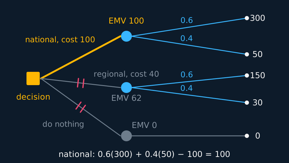
A decision node, drawn as a square, is a point where you choose. A chance node, drawn as a circle, is a point where the world chooses, with probabilities on the branches. Pay-offs go at the ends, and any cost incurred along a branch is subtracted at the point it is met.
Working back, a chance node takes the expected monetary value of its branches, which is the probability-weighted average. A decision node retains the greatest value available under the criterion in use, and the rejected branches are struck through. Repeating this back to the first decision gives the action with the greatest EMV, together with the working that justifies it.
Under the expected monetary value criterion, choose the action with the greatest EMV. A decision-maker may choose differently when utility, risk tolerance or an unacceptable adverse outcome is relevant.
Describe the drawing
A decision tree with a square decision node on the left, three branches carrying their costs, and a chance node on each of the two launches. From each chance node two probability-labelled branches, 0.6 and 0.4, lead to terminal payoffs of 300 and 50 for national and 150 and 30 for regional; doing nothing pays 0. Rolling back gives expected monetary values of 100, 62 and 0, the national branch is drawn heavily, and the two rejected branches are struck through with double ticks.
WORKED EXAMPLE
Choosing a launch
A product can be launched nationally, costing 100, with a 0.6 chance of revenue 300 and 0.4 of 50; regionally, costing 40, with 0.6 of 150 and 0.4 of 30; or not at all. All figures in thousands. Which is best on expected monetary value?
National: 0.6(300) + 0.4(50) − 100 = 180 + 20 − 100 = 100.
Regional: 0.6(150) + 0.4(30) − 40 = 90 + 12 − 40 = 62.
Doing nothing: 0.
The national launch has the greatest expected monetary value, so it is the choice under the EMV criterion.
Limitations of expected monetary value
Expected monetary value is a long-run average over many repetitions, and a one-off decision is not many repetitions. A firm that would be ruined by the adverse outcome may prefer a smaller certain gain. The criterion supplies a number; it does not by itself settle the decision.
Utility replaces money with a measure of how much each outcome is worth to the decision-maker. For a risk-averse decision-maker that measure rises less than proportionally with money. Maximising expected utility can then favour the safer option even where the expected monetary value is lower, which is the appropriate treatment when the stakes are large compared with the resources available.
GUIDED PRACTICE
Reading the risk
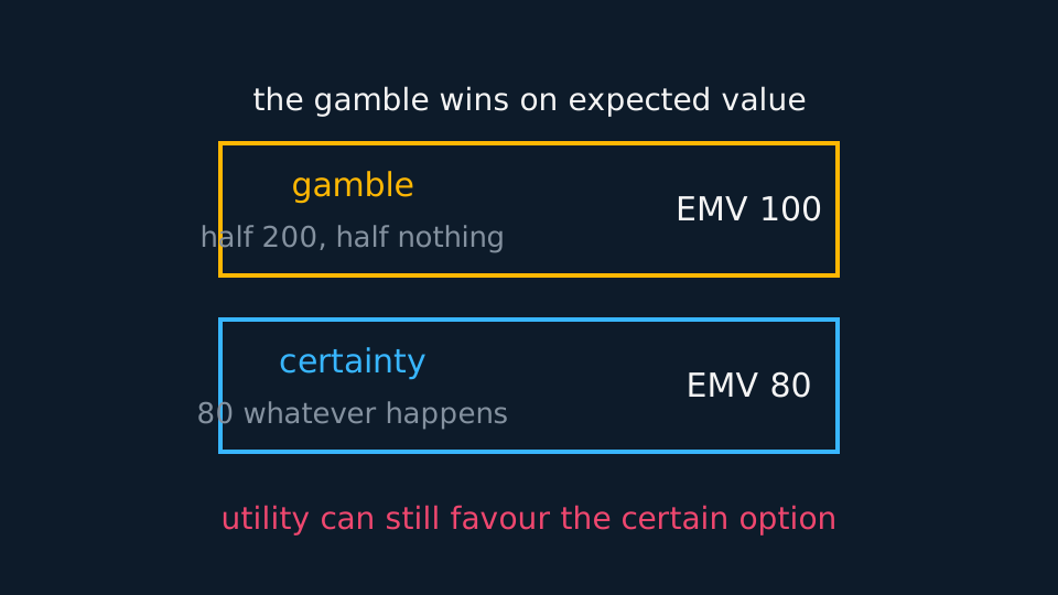
In the launch example, a competitor offers to buy the product outright for 80 thousand. Compare the options and comment.
Show the working
The certain sale is worth 80, against the national launch's expected 100.
On expected monetary value the launch wins by 20.
But the launch has a 0.4 chance of returning only 50 against a cost of 100, a loss of 50.
A firm that could not absorb that loss should take the 80. The expected monetary value calculation is correct and still not the whole answer.
ASSESSMENT FOCUS
- Use squares for decision nodes and circles for chance nodes, and label every probability.
- Subtract costs along the branch where they are incurred, not at the end.
- Write the expected monetary value at each chance node, mark the rejected branches and record the retained value at each decision node.
- Say which criterion the choice is made under: an EMV answer is best under the EMV criterion, not best without qualification.
CHECK YOURSELF
A chance node has a 0.3 branch paying 200 and a 0.7 branch paying 50, and reaching it costs 60. Find the expected monetary value.
Show a hint
Average the branches, then subtract the cost.
Show the answer
0.3(200) + 0.7(50) = 60 + 35 = 95, and subtracting the cost of 60 leaves an expected monetary value of 35.
Chance nodes take the probability-weighted average and decision nodes retain the greatest value under the criterion in use, worked back to the first decision.
Expected monetary value is an average over repetitions, so for a one-off decision with large stakes utility may favour the safer option.
WORKBOOK
Printable practice for this topic: original exam-style questions with room to work, and a fully worked answer book. Free to use; please do not redistribute or sell.
Or read them with their worked answers on the decision trees, expected monetary value and utility questions page.
CHECK YOUR PROGRESS
Rate how confident you feel with each objective for this lesson. Ratings are saved in this browser, on this device, unless you sign in.
- Draw a decision tree and work expected monetary values back to the first decision.
- Explain the limits of expected monetary value and where utility helps.
Open the full revision checklist to see every objective in the course in one place.