Maths › Decision Mathematics 2 › Mixed strategies in game theory
Mixed strategies in game theory
When a game has no pure saddle point, each player does best with a mixed strategy, randomising between choices in fixed proportions. The graphical method applies to a 2 × n or n × 2 game, where the optimal proportion is read from the highest point of the lower boundary; larger games are formulated as linear programmes.
Builds on Game theory: play safe and stable solutions and The Simplex algorithm.
IN THIS TOPIC
- Set up the expected pay-off against each opposing choice as a function of p.
- Solve a 2 by n or n by 2 game graphically and state the value, and formulate a larger game as a linear programme.
- Convert a larger game into a linear program for Simplex.
COMMON MISCONCEPTION
In a mixed strategy the player should favour the choice with the larger pay-offs, in proportion to them.
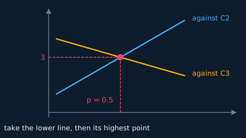
Geometry sets the proportions, not the sizes of the pay-offs. Write the expected pay-off against each opposing choice as a line in p, and the best mix is the highest point of the lower boundary, a crossing or an end. Rows (5, 2) and (1, 4) give 1 + 4p and 4 − 2p, which cross at p = 0.5 for a value of 3, so the two rows are played equally often although their entries are not equal.
Graphical solution for a 2 × n game
Suppose the row player plays R1 with probability p and R2 with probability 1 − p. Against each column the expected pay-off is a linear function of p, so plotting them over 0 ≤ p ≤ 1 gives one straight line per column.
Whatever p is, the row player is guaranteed at least the lowest of those lines, so the best p is where that lower boundary reaches its highest point. The boundary is a chain of straight pieces that only ever bends downwards, so its highest point sits either at a corner, where two lines cross, or at an end, p = 0 or p = 1. Those are the candidates, and both kinds have to be checked. Equate the pair meeting at the winning corner for p, then substitute to get the value of the game.
Rows (5, 3) and (1, 2) show why the ends are on the list. The lines are 1 + 4p and 2 + p, crossing at p = 1/3 where the guarantee is only 7/3. Both lines rise, so the boundary keeps rising to p = 1, where the guarantee is the better 3. Equating the crossing without looking at the ends would have quoted 7/3 for a game worth 3. The warning sign was there earlier: R1 gives a better pay-off than R2 in both columns, so R2 was dominated and should have gone before any line was drawn. An optimum at an end always means a pure strategy, and usually means a dominated row survived the reduction.
WORKED EXAMPLE
Solving a two by two game
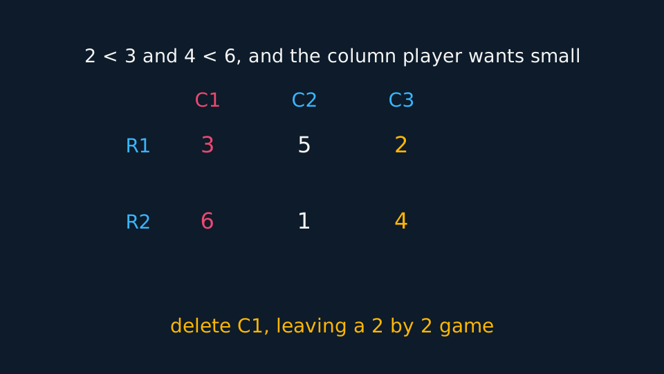
After deleting a dominated column, a game has rows (5, 2) and (1, 4). Find the row player's optimal mix and the value.
Against the first column: 5p + 1(1 − p) = 1 + 4p. Against the second: 2p + 4(1 − p) = 4 − 2p.
Equating: 1 + 4p = 4 − 2p, so 6p = 3 and p = 0.5.
The value is 1 + 4(0.5) = 3, and the other expression gives 4 − 1 = 3 as a check. The row player plays each row half the time.
The column player's side
The column player's mix is found the same way, plotting expected losses against each row and taking the lowest point of the upper boundary. The value comes out the same, which makes it a useful check.
For a 2 by n or n by 2 game, plot all n lines and read off the highest point of the lower boundary. Equate the pair that meets there and say from the graph which pair you are using; equating the wrong pair is the standard loss of marks in this topic.
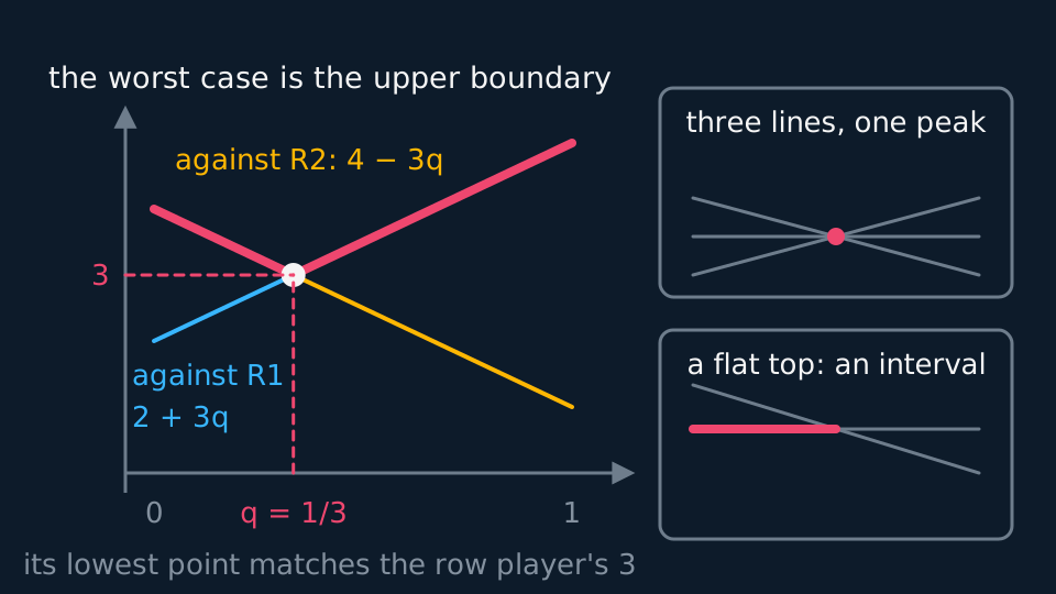
Three situations are worth recognising before you start equating. If three or more lines pass through the peak, any two boundary pieces meeting there give the same p and the same value, so pick the easiest pair and say which. If a boundary piece is flat at the peak, every p across that stretch is optimal and the game has an interval of best mixes rather than one; quote the interval and name a member of it. And if the peak is at p = 0 or p = 1, no equating is needed: the optimum is the pure strategy at that end, with the value read straight off the lowest line there.
Describe the drawing
The column player's two expected-loss lines plotted against the probability q of the first column, one rising and one falling, with the upper stretch of the pair drawn thick. That worst-case boundary is lowest where the lines cross, at q of one third and a loss of three, the same value the row player found. Two small inset panels show the shapes to watch for: three lines passing through a single peak, where any two of them give the same answer, and a boundary with a flat piece, where a whole interval of mixes is optimal.
GUIDED PRACTICE
The column player's mix
For the same two by two game, find the column player's optimal mix and confirm the value.
Show the working
Let the column player play C1 with probability q. Against R1 the expected loss is 5q + 2(1 − q) = 2 + 3q.
Against R2 it is 1q + 4(1 − q) = 4 − 3q.
Equating: 2 + 3q = 4 − 3q, so 6q = 2 and q = 1/3.
The value is 2 + 1 = 3, agreeing with the row player's calculation, so both mixes are correct.
Linear-programming formulation
The graphical method applies to a 2 × n or n × 2 game, because one player then has two strategies and a single probability p describes the mix. If both players retain more than two strategies, formulate the game as a linear programme. Write p1, p2, ... for the row player's probabilities and V for the value. Each column gives one constraint saying the expected pay-off against it is at least V, and the probabilities add to 1.
Simplex needs everything non-negative, so add a constant to every entry first if any are negative, which raises the value by that constant and changes nothing else. Maximise V, solve the tableau, and subtract the constant again at the end to recover the true value.
ASSESSMENT FOCUS
- Define p clearly as the probability of one named row, and say which.
- Write the expected pay-off against every opposing choice as a function of p.
- Equate only the two expressions that meet at the optimum, and justify which those are from the graph.
- Check the ends, p = 0 and p = 1, alongside the crossings. A boundary that peaks at an end means a pure strategy, and usually a dominated row you did not delete.
- Check the value by working out the other player's mix as well.
CHECK YOURSELF
Against two columns the expected pay-offs are 2 + 5p and 7 − 3p. Find the optimal p and the value.
Show a hint
Equate the two.
Show the answer
2 + 5p = 7 − 3p gives 8p = 5, so p = 0.625. The value is 2 + 5(0.625) = 5.125, and 7 − 3(0.625) = 5.125 confirms it.
Plot the expected pay-off against each opposing choice as a line in p; the optimum is the highest point of the lower boundary, which is a crossing or an end.
Equate the pair meeting there for p and the value, test p = 0 and p = 1 too, and check against the other player's mix; the method covers 2 × n and n × 2 games, and larger ones are formulated as linear programmes.
WORKBOOK
Printable practice for this topic: original exam-style questions with room to work, and a fully worked answer book. Free to use; please do not redistribute or sell.
Or read them with their worked answers on the mixed strategies in game theory questions page.
CHECK YOUR PROGRESS
Rate how confident you feel with each objective for this lesson. Ratings are saved in this browser, on this device, unless you sign in.
- Set up the expected pay-off against each opposing choice as a function of p.
- Solve a 2 by n or n by 2 game graphically and state the value, and formulate a larger game as a linear programme.
- Convert a larger game into a linear program for Simplex.
Open the full revision checklist to see every objective in the course in one place.