Maths › Decision Mathematics 2 › The stepping-stone method
The stepping-stone method
Shadow costs and improvement indices identify which unused route would reduce the total cost of a transportation plan. The stepping-stone method then moves goods onto that route while keeping every row and column total intact.
Builds on Transportation problems and The Simplex algorithm.
IN THIS TOPIC
- Find shadow costs from the cells in use.
- Compute improvement indices and identify the entering cell.
- Trace the stepping-stone route, find the exiting cell, and state the new cost.
- Formulate a transportation problem as a linear program.
- Add a zero allocation when too few cells are in use for the shadow costs.
COMMON MISCONCEPTION
The entering cell is the unused cell with the lowest cost in the table.
The entering cell is the unused cell with the most negative improvement index, cost − R − K, where R and K are the row and column shadow costs. A raw cost says nothing about the goods elsewhere in the plan that would have to shift to accommodate the new route. A cell costing 3, the cheapest in the table, can carry a positive index while one costing 9 carries −2 and enters.
Shadow costs and indices
Give each row a number R and each column a number K, chosen so that R + K equals the cost of every cell currently in use. Setting the first R to zero fixes all the rest, and the m + n − 1 cells in use are exactly enough to determine them.
The formulae booklet carries nothing at all for Decision Maths, so every definition and every algorithm in this unit has to come from memory. A negative index means that route is cheaper than the shadow costs predict, so sending goods along it would reduce the total. The most negative index gives the entering cell. It need not be the cheapest unused cell in the table, because a raw cost says nothing about everything else in the plan that would have to shift to accommodate it, and shifting is what the shadow costs measure.
WORKED EXAMPLE
Which cell enters
For the north-west corner solution, find the shadow costs and the improvement indices.
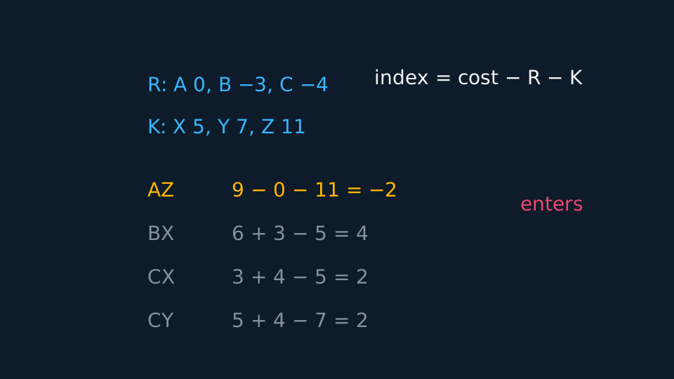
Setting RA = 0: AX in use gives KX = 5, AY gives KY = 7, BY gives RB = −3, BZ gives KZ = 11, and CZ gives RC = −4.
Indices: AZ = 9 − 0 − 11 = −2; BX = 6 + 3 − 5 = 4; CX = 3 + 4 − 5 = 2; CY = 5 + 4 − 7 = 2.
Only AZ is negative, so AZ enters. Note that CX has the lowest cost in the whole table at 3, yet its index is positive.
Moving goods round the loop
From the entering cell, trace a closed route through cells already in use, alternately adding and subtracting. Each row and column must gain as much as it loses, which is what keeps the supplies and demands satisfied. Mark the entering cell with a plus and alternate round the loop.
The quantity moved, θ, is the smallest allocation sitting in a minus cell, since anything larger would drive that cell negative. That cell empties and becomes the exiting cell. The new cost is the old one plus θ times the improvement index, and it is worth checking that against a direct recalculation of the whole table.
GUIDED PRACTICE
One improvement
Carry out the improvement on the entering cell AZ, and state the new cost.
Show the working
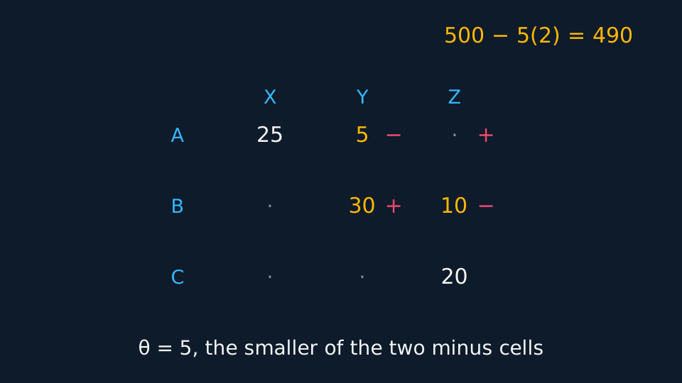
The loop is AZ plus, AY minus, BY plus, BZ minus, back to AZ.
The minus cells hold AY 5 and BZ 10, so θ = 5 and AY exits.
New allocations: AX 25, AZ 5, BY 35, BZ 5, CZ 20.
New cost = 500 + 5(−2) = 490, and recalculating directly gives 125 + 45 + 140 + 40 + 140 = 490. A further round of indices shows none negative, so 490 is optimal.
The same problem as a linear program
Write xij for the number of units sent from source i to destination j. Minimise the total cost Σ cijxij, subject to one equation per source saying its shipments add to its supply, one equation per destination saying its receipts add to its demand, and xij ≥ 0 throughout.
A 3 by 3 problem therefore has nine variables and six constraints, one of which is redundant once the problem is balanced. Simplex would solve it, slowly. The transportation method is that same algorithm specialised to this shape, and that kinship is why shadow costs behave so much like the objective row of a tableau.
ASSESSMENT FOCUS
- Set the first shadow cost to zero and say that you have done so.
- Compute an index for every unused cell, not only the ones you expect to be negative.
- Draw the stepping-stone loop on the table with the plus and minus signs marked.
- State θ, name the exiting cell, and check the new cost two ways.
- Stop when no index is negative, and say that is why you have stopped.
CHECK YOURSELF
An unused cell has cost 12, its row shadow cost is 4 and its column shadow cost is 9. Find the improvement index and say what it means.
Show a hint
Cost minus the two shadow costs.
Show the answer
12 − 4 − 9 = −1. The index is negative, so using this route would reduce the total cost by 1 for every unit sent along it, and the cell is a candidate to enter.
Shadow costs satisfy R + K = cost for every cell in use, and the improvement index of an unused cell is cost − R − K.
The most negative index enters; θ is the smallest minus-cell allocation, that cell exits, and the cost changes by θ times the (negative) index.
As a linear program, minimise Σ c x subject to one equation per source and one per destination.
WORKBOOK
Printable practice for this topic: original exam-style questions with room to work, and a fully worked answer book. Free to use; please do not redistribute or sell.
Or read them with their worked answers on the stepping-stone method questions page.
CHECK YOUR PROGRESS
Rate how confident you feel with each objective for this lesson. Ratings are saved in this browser, on this device, unless you sign in.
- Find shadow costs from the cells in use.
- Compute improvement indices and identify the entering cell.
- Trace the stepping-stone route, find the exiting cell, and state the new cost.
- Formulate a transportation problem as a linear program.
- Add a zero allocation when too few cells are in use for the shadow costs.
Open the full revision checklist to see every objective in the course in one place.