Maths › Further Statistics 1 › Contingency tables
Contingency tables
A contingency table cross-tabulates two categorical variables, and a chi-squared test assesses whether they are independent. Expected counts come from the row and column totals and the degrees of freedom from the shape of the table. On a two by two table, OCR H245 requires Yates' correction; AQA 7367 expects you to know when and how to apply it.
Builds on Goodness-of-fit tests and Conditional probability.
IN THIS TOPIC
- Compute expected frequencies as row total × column total ÷ grand total.
- Use (rows − 1)(columns − 1) degrees of freedom.
- Merge rows or columns whose expected frequency falls below the stated condition, and recount the degrees of freedom from the merged table.
- State the hypotheses as independence and association, and conclude in context.
- Apply Yates' correction to a two by two table where the specification requires it, and say why it is used.
- Form the chi-squared statistic from the cell contributions (O − E)²/E, and read the largest contributions and their signs when interpreting the result.
COMMON MISCONCEPTION
Expected frequencies in a contingency table come from assuming every cell is equally likely.
The null hypothesis is that the two variables are independent, not that the cells are equal. Under independence the probability of a cell is the product of its row and column probabilities, so its expected frequency is row total times column total divided by grand total. A row holding twice as many observations expects twice as much in every column.
Expectations from the margins
The null hypothesis is that the two variables are independent. It is not that the cells are equal. Under independence the probability of a cell is the product of its row and column probabilities, so multiplying by the grand total gives:
Pearson Edexcel 9FM0 formulae booklet: the χ² statistic is included, this expression for an expected frequency is not. A row holding twice as many observations expects twice as much in every column, which is what the formula gives.
Describe the drawing
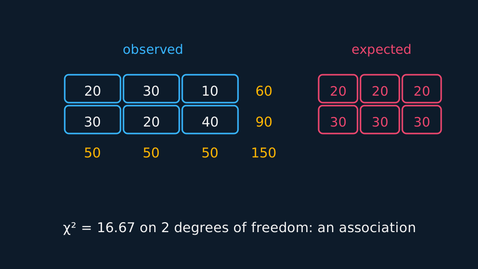
Two grids side by side. The cyan one holds the observed counts with amber row and column totals; the coral one holds the expected counts under independence, twenty across the smaller row and thirty across the larger. The gaps between them give a chi-squared of sixteen point six seven on two degrees of freedom.
Each cell then contributes the square of its difference from expectation, divided by that expectation, and the statistic is the total of those contributions across the table:
WORKED EXAMPLE
Testing an association
A survey cross-tabulates two variables as rows (20, 30, 10) and (30, 20, 40). Test at the 5% level whether the variables are independent.
H₀: there is no association between the two variables. H₁: there is an association.
Row totals 60 and 90; column totals 50, 50, 50; grand total 150. Expected: 60 × 50/150 = 20 across the first row, and 30 across the second.
χ² = 0 + 5 + 5 + 0 + 3.33 + 3.33 = 16.67.
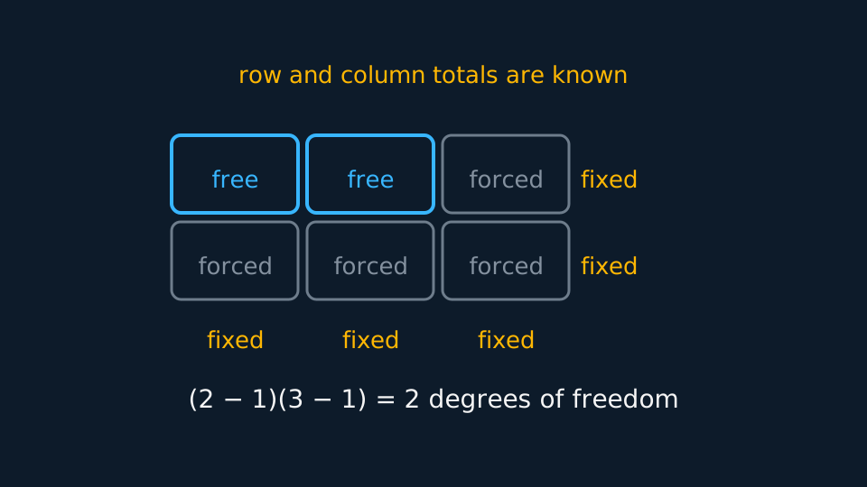
Degrees of freedom (2 − 1)(3 − 1) = 2, critical value 5.991.
16.67 > 5.991, so reject H₀. There is evidence at the 5% level of an association between the two variables.
Degrees of freedom and interpretation
Once the margins are fixed, filling in one cell of a 2 × 2 table forces every other. In general only (rows − 1)(columns − 1) cells are free, and that count is the degrees of freedom. Nothing is subtracted for estimated parameters here, because the margins have already absorbed them.
Examine the individual contributions before writing the conclusion. In the example above the first column contributes nothing, while the four cells of the other two columns contribute between 3.33 and 5 each. The association therefore arises from how those two categories split between the rows. In an interpretation, name the largest contributor and state the direction in which that cell departs from its expected frequency.
GUIDED PRACTICE
Degrees of freedom before and after pooling
A contingency table has 4 rows and 3 columns, with no expected frequency below 5. State the degrees of freedom. Then state them again for the case where two of the rows have to be combined.
Show the working
As it stands: (4 − 1)(3 − 1) = 6 degrees of freedom.
Combining two rows leaves 3 rows: (3 − 1)(3 − 1) = 4.
Pooling always costs degrees of freedom, since it removes cells that were free to vary.
The two by two case, and Yates' correction
A table with two rows and two columns is the smallest there is, and it carries a single degree of freedom. With the margins fixed, one cell settles the other three, so the four differences O − E come out the same size and alternate in sign, and the statistic rests on that one number. The χ² distribution, however, is a continuous curve used to describe a statistic that moves in jumps, because the counts are whole numbers. On one degree of freedom the mismatch leans one way: the statistic comes out a little large, so the test rejects the null hypothesis more readily than the stated 5% suggests.
Yates' correction pulls each difference half a unit towards zero before it is squared:
It is the same continuity correction used when a discrete count is read against a continuous normal curve, applied here to the one table shape where the approximation is weakest. Apply it to a two by two table and not to a larger one. Subtracting the half reduces the statistic whenever the differences are large enough to be worth testing, so the correction moves a conclusion towards not rejecting the null hypothesis rather than away from it.
Board scope. AQA 7367 and Cambridge OCR H245: know when and how to apply Yates' correction to a 2 × 2 contingency table, OCR H245 requiring it for that case. Pearson Edexcel 9FM0: this correction is not listed in the Further Statistics content, so check the current specification before applying it in a 9FM0 answer.
The correction repairs an approximation rather than improving the statistic, and statisticians disagree about it: on some tables it overcorrects and makes the test too cautious, and for small counts Fisher's exact test is preferred. Where the correction is required, state that the table has one degree of freedom and show one corrected contribution in full.
WORKED EXAMPLE
A conclusion that turns on the correction
Of 100 commuters, 50 live within two miles of work and 50 further away. Among the nearer group 30 cycle; among the further group 20 do. Test at the 5% level for an association between distance and cycling.
H₀: distance and cycling are independent. H₁: they are associated.
The margins are 50 throughout, so each expected frequency is 50 × 50/100 = 25, and the four differences are 5 in size.
Uncorrected: χ² = 4 × 5²/25 = 4.00, against a critical value of 3.841 on one degree of freedom.
Corrected: each contribution is (5 − 0.5)²/25 = 20.25/25 = 0.81, so χ² = 4 × 0.81 = 3.24.
3.24 < 3.841, so do not reject H₀: there is insufficient evidence at the 5% level of an association between distance and cycling. The uncorrected statistic would have reached the opposite conclusion, which is why the correction has to be stated where a specification requires it.
GUIDED PRACTICE
A corrected statistic on uneven margins
A trial records 40 people on a new scheme, of whom 24 passed, and 60 on the old scheme, of whom 21 passed. Apply Yates' correction and test at the 5% level.
Show the working
Margins: rows 40 and 60, columns 45 passes and 55 failures, total 100. Expected frequencies 18 and 22 on the top row, 27 and 33 on the bottom.
Each |O − E| is 6, so each corrected numerator is 5.5² = 30.25.
Contributions 30.25/18 = 1.681, 30.25/22 = 1.375, 30.25/27 = 1.120 and 30.25/33 = 0.917, giving χ² = 5.09 to three significant figures.
5.09 > 3.841 on one degree of freedom, so reject H₀: there is evidence at the 5% level of an association between scheme and outcome. Here the correction changed the statistic, which was 6.06 without it, and left the conclusion standing.
ASSESSMENT FOCUS
- Write the hypotheses as 'no association' against 'some association', naming both variables.
- Compute expected frequencies to one decimal place and show at least one of them in full.
- Degrees of freedom are (r − 1)(c − 1). Do not subtract again for estimated parameters.
- Check the expected-frequency condition your specification states. Combine categories only where the combined category remains meaningful; otherwise the chi-squared approximation may be unsuitable and a different test may be needed.
- On a two by two table, apply Yates' correction where the specification requires it, and show one corrected contribution in full.
CHECK YOURSELF
A contingency table has 3 rows and 4 columns. State the degrees of freedom, and find the expected frequency for a cell whose row total is 40 and column total is 30, with grand total 200.
Show a hint
(r − 1)(c − 1), and row × column ÷ total.
Show the answer
Degrees of freedom (3 − 1)(4 − 1) = 6. Expected frequency 40 × 30/200 = 6.
Expected = row total × column total ÷ grand total, which is independence written as arithmetic.
Degrees of freedom are (rows − 1)(columns − 1), because the margins have already used up the rest.
On a two by two table, where one degree of freedom makes the continuous approximation weakest, OCR H245 requires 0.5 to be subtracted from each |O − E| before squaring, and AQA 7367 expects you to know when to do so.
WORKBOOK
Printable practice for this topic: original exam-style questions with room to work, and a fully worked answer book. Free to use; please do not redistribute or sell.
Or read them with their worked answers on the contingency tables questions page.
CHECK YOUR PROGRESS
Rate how confident you feel with each objective for this lesson. Ratings are saved in this browser, on this device, unless you sign in.
- Compute expected frequencies as row total × column total ÷ grand total.
- Use (rows − 1)(columns − 1) degrees of freedom.
- Merge rows or columns whose expected frequency falls below the stated condition, and recount the degrees of freedom from the merged table.
- State the hypotheses as independence and association, and conclude in context.
- Apply Yates' correction to a two by two table where the specification requires it, and say why it is used.
- Form the chi-squared statistic from the cell contributions (O − E)²/E, and read the largest contributions and their signs when interpreting the result.
Open the full revision checklist to see every objective in the course in one place.