Maths › Further Statistics 1 › Goodness-of-fit tests
Goodness-of-fit tests
A goodness-of-fit test compares a model's predicted frequencies with the observed ones. The chi-squared statistic measures the mismatch, and comparing it with a critical value shows whether it is larger than chance alone would produce.
Builds on Hypothesis tests for Poisson and geometric models and Representing and interpreting data.
IN THIS TOPIC
- Compute expected frequencies from a proposed model and form the χ² statistic.
- Count degrees of freedom, subtracting one for each estimated parameter.
- Pool classes whose expected frequency falls below the stated condition, then recount the classes.
- Fit and test a Poisson or binomial model from start to finish.
- Build expected frequencies for a continuous model from the probability of each class interval.
- State the hypotheses, compare χ² with the critical value, and conclude in the language of evidence.
COMMON MISCONCEPTION
A large chi-squared statistic proves the model is wrong; a small one proves it is right.
The test proves nothing in either direction. It compares the statistic with a critical value on the degrees of freedom left after pooling, one fewer for each parameter estimated from the data, and reports evidence: a large value is evidence against the model, and a small one leaves insufficient evidence to reject it.
The chi-squared statistic
Multiply each class's model probability by the total to get its expected frequency, then accumulate:
Pearson Edexcel 9FM0 formulae booklet: included, under Non-parametric tests, for goodness-of-fit and contingency tables alike, with percentage points of χ² tabulated separately. Squaring makes over- and under-shoots count alike. Dividing by E makes a gap of 3 in a class expecting 5 count for far more than the same gap in a class expecting 500. A large value means the model fits badly. The test never proves anything either way, since it only compares the statistic with a critical value and reports evidence.
WORKED EXAMPLE
Is the die fair?
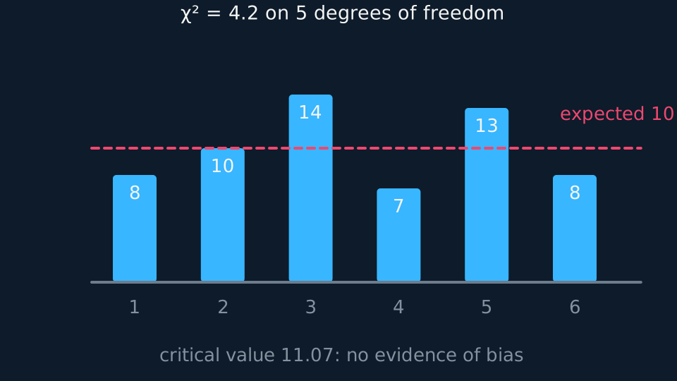
A die is thrown 60 times, giving 8, 10, 14, 7, 13, 8. Test at the 5% level whether it is fair.
H₀: the die is fair, so each expected frequency is 10. H₁: the die is not fair.
χ² = (4 + 0 + 16 + 9 + 9 + 4)/10 = 4.2.
Degrees of freedom: 6 classes − 1 = 5, and the 5% critical value is 11.07.
4.2 < 11.07, so do not reject H₀. There is insufficient evidence at the 5% level that the die is unfair.
Degrees of freedom and pooling
Start with the number of classes. Subtract 1, because the frequencies must total the sample size. Then subtract 1 more for every parameter estimated from the data. Fitting a Poisson model with λ taken from the sample mean costs a degree of freedom. Fitting one with λ specified in advance does not. A binomial with both n and p given costs nothing extra; a binomial with p estimated costs one.
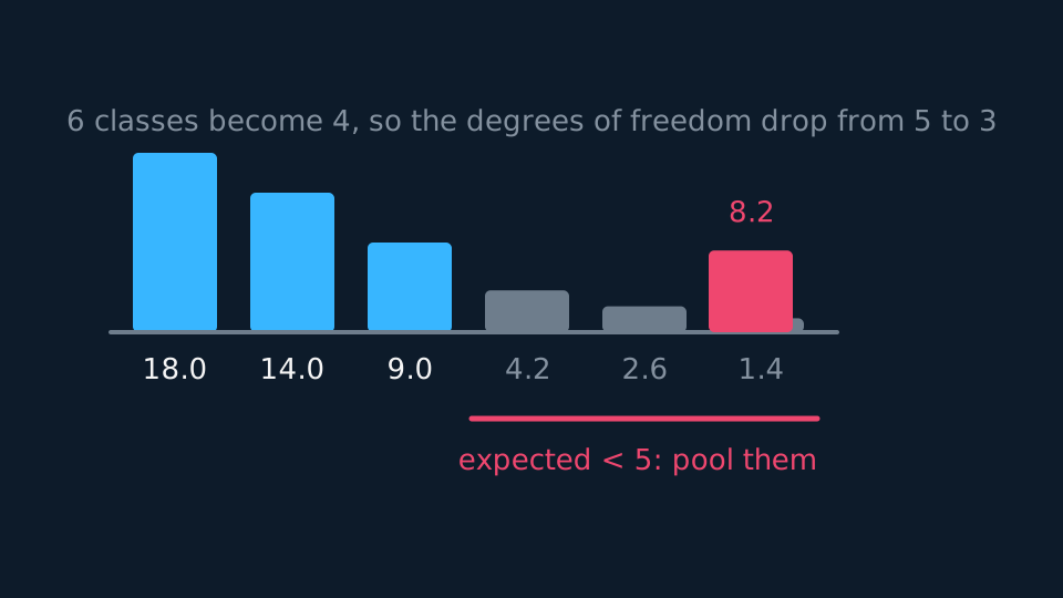
Small expected frequencies weaken the chi-squared approximation, so small classes are pooled with their neighbours before the statistic is computed. Check the expected-frequency condition your specification states; Pearson Edexcel 9FM0 uses a minimum expected frequency of 5. Combine classes only where the combined class remains meaningful; otherwise the approximation may be unsuitable and a different test may be needed. Pooling is a separate step from estimating parameters: the class count used for the degrees of freedom is the pooled one, and each estimated parameter then removes one further degree of freedom.
GUIDED PRACTICE
Degrees of freedom under two regimes
A Poisson model is fitted to data in 7 classes after pooling. Give the degrees of freedom when λ is specified in advance, and when λ is estimated from the sample mean.
Show the working
Specified in advance: 7 − 1 = 6 degrees of freedom.
Estimated from the data: 7 − 1 − 1 = 5.
Estimating a parameter lets the model bend towards the data, so one degree of freedom is surrendered to pay for the flexibility.
A Poisson fit from start to finish
A complete fit runs in four steps: estimate λ from the data, build the expected frequencies, pool the tail, then test. Work down the table in one pass and keep the expected values to two decimal places until the final statistic.
Read the last row of the observed table before totalling anything. A table that stops at a stated value, four flaws here, records exactly how many events there were, so the sample mean is available and the fitted λ is that mean. A table whose last row reads '4 or more' does not. Counting each of those observations as a bare 4 gives a lower bound for the total and a lower bound for λ, never the mean, and every expected frequency built on it inherits that bias. In that case the total or λ itself must be supplied. The model's final class is 'x or more' either way, because probability leaks past the largest value seen and the expected frequencies must total n.
WORKED EXAMPLE
Flaws in a batch of components
The number of flaws in each of 100 components is recorded as 30 with none, 36 with one, 21 with two, 10 with three and 3 with four. Test at the 5% level whether a Poisson model fits.
The sample mean is 120/100 = 1.2, so fit Po(1.2). H₀: a Poisson distribution is a suitable model. H₁: it is not.
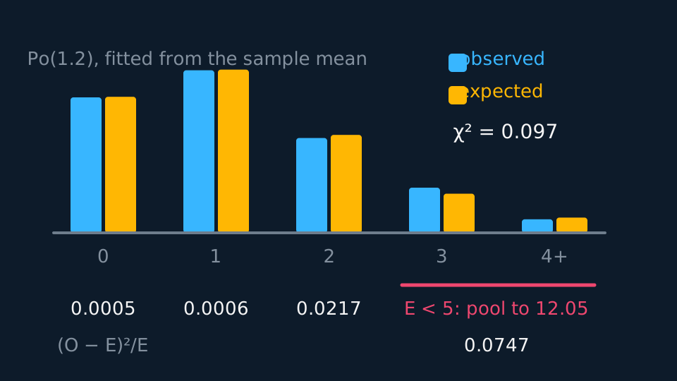
Expected frequencies from Po(1.2), with the last class taken as '4 or more': 30.12, 36.14, 21.69, 8.67, 3.38.
The last expects 3.38, below 5, so pool it with the class before. That leaves four classes: 0, 1, 2 and '3 or more', with observed 30, 36, 21, 13 against expected 30.12, 36.14, 21.69, 12.05.
χ² = 0.0005 + 0.0006 + 0.0217 + 0.0747 = 0.097.
λ was estimated, so the degrees of freedom are 4 − 1 − 1 = 2, and the 5% critical value is 5.991.
0.097 < 5.991, so do not reject H₀. There is insufficient evidence at the 5% level against a Poisson model for the flaws.
Describe the drawing
Five pairs of bars compare the observed flaw counts with the expected frequencies from a fitted Poisson of mean one point two, and the pairs are almost the same height everywhere. The last class expects only three point four, below five, so a coral bracket pools it with its neighbour into a class expecting twelve point nought five. Each surviving cell's squared gap over its expectation is printed beneath it, and the four contributions add to the tiny statistic nought point nought nine seven.
When the model is continuous
The fits above are all to discrete models, where a class is a single value and its probability is read straight off the distribution. A continuous model attaches no probability to a value, so a class has to be an interval and its probability is the area under the density across it, which is F(b) − F(a) for a class running from a to b. Multiply that by the total for the expected frequency, and the rest of the test proceeds unchanged: pool anything under 5, count the classes that survive, subtract for estimated parameters.
Two points of care. The outer classes are opened out to run to −∞ and to +∞, or the probabilities total less than 1 and the expected frequencies total less than n. And the boundaries used are the true ones: masses recorded to the nearest gram in a class labelled 45 to 49 occupy 44.5 to 49.5, and the model probability is taken between those. A normal model whose mean and standard deviation are both estimated from the grouped data costs two degrees of freedom, one for each.
WORKED EXAMPLE
A normal model for 200 masses
The masses of 200 items in grams are grouped as: under 42.5, 10 items; 42.5 to 47.5, 52; 47.5 to 52.5, 78; 52.5 to 57.5, 46; over 57.5, 14. Test at the 5% level whether N(50, 5²) fits, the parameters having been specified in advance.
H₀: N(50, 5²) is a suitable model. H₁: it is not.
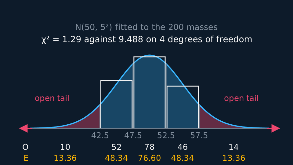
Standardising the four interior boundaries gives z = −1.5, −0.5, 0.5 and 1.5, and the tables give Φ as 0.0668, 0.3085, 0.6915 and 0.9332.
Differencing, with the outer classes run to infinity, the class probabilities are 0.0668, 0.2417, 0.3830, 0.2417, 0.0668, which total 1 as they should.
Multiplying by 200: expected frequencies 13.36, 48.34, 76.60, 48.34, 13.36. None is below 5, so nothing is pooled.
χ² = 0.845 + 0.277 + 0.026 + 0.113 + 0.031 = 1.29.
Both parameters were given, so the degrees of freedom are 5 − 1 = 4 and the 5% critical value is 9.488.
1.29 < 9.488, so do not reject H₀. There is insufficient evidence at the 5% level against a normal model with mean 50 and standard deviation 5.
Had the two parameters been estimated from the grouped data instead, the degrees of freedom would be 5 − 1 − 2 = 2 and the critical value 5.991. The conclusion would be unchanged here, because 1.29 is below both critical values.
Opening the two outer classes to −∞ and +∞ is what makes the five class probabilities total 1. Each observed bar is close to the expected frequency under the fitted curve, which is why the statistic is small.
Describe the drawing
A normal curve of mean fifty and standard deviation five drawn over the 200 masses, with the three middle classes outlined as histogram bars of fifty-two, seventy-eight and forty-six. The area under the curve is divided at forty-two point five, forty-seven point five, fifty-two point five and fifty-seven point five, and the two outer areas are left open, running off the ends of the axis so that the five probabilities total one. Multiplying them by two hundred gives the expected frequencies printed beneath: thirteen point three six, forty-eight point three five, seventy-six point five nine, forty-eight point three five and thirteen point three six, which total two hundred. The bars and the areas are close everywhere, and the test statistic of one point two nine falls far short of nine point four eight eight.
GUIDED PRACTICE
A continuous uniform fit
120 waiting times in minutes are grouped as: 0 to 10, 26 times; 10 to 30, 34; 30 to 45, 31; 45 to 60, 29. Test at the 5% level whether a continuous uniform distribution on 0 to 60 fits, given a critical value of 7.815.
Show the working
H₀: the times are uniformly distributed on 0 to 60. H₁: they are not. For a uniform density the probability of a class is its width over 60: 1/6, 1/3, 1/4 and 1/4, totalling 1.
Expected frequencies: 20, 40, 30, 30. All are at least 5, so no pooling is needed.
χ² = 36/20 + 36/40 + 1/30 + 1/30 = 1.8 + 0.9 + 0.033 + 0.033 = 2.77.
No parameter was estimated, so there are 4 − 1 = 3 degrees of freedom. Since 2.77 < 7.815, do not reject H₀: there is insufficient evidence at the 5% level against a uniform model.
The unequal class widths cost nothing here, because the probability of a class under a uniform density is proportional to its width.
ASSESSMENT FOCUS
- Compute expected frequencies to at least two decimal places before squaring anything.
- First pool classes below the expected-frequency condition your specification states, then count classes for the degrees of freedom.
- Subtract one degree of freedom for every parameter estimated from the data, and name which parameter.
- For a geometric or Poisson fit, the final class is 'x or more' and its probability is 1 minus everything before it.
- For a continuous model, take each class probability as F(upper) − F(lower), and run the two outer classes out to infinity so the probabilities total 1.
- Use true class boundaries for a continuous fit: a class labelled 45 to 49 for data rounded to the nearest unit runs from 44.5 to 49.5.
- Conclude with evidence language. 'Insufficient evidence to reject' is the phrase; 'the model is correct' is not.
CHECK YOURSELF
A goodness-of-fit test uses 5 classes after pooling, with the distribution's single parameter estimated from the data. State the degrees of freedom.
Show a hint
Classes minus one, minus one per estimated parameter.
Show the answer
5 − 1 − 1 = 3 degrees of freedom.
χ² sums (O − E)²/E, so each squared gap is weighted down by how large its class was expected to be.
Degrees of freedom are classes minus 1, minus one more for each parameter estimated from the data, counted after pooling.
A discrete model gives a class its probability at a point; a continuous one gives it F(upper) − F(lower), with the outer classes run to infinity.
WORKBOOK
Printable practice for this topic: original exam-style questions with room to work, and a fully worked answer book. Free to use; please do not redistribute or sell.
Or read them with their worked answers on the goodness-of-fit tests questions page.
CHECK YOUR PROGRESS
Rate how confident you feel with each objective for this lesson. Ratings are saved in this browser, on this device, unless you sign in.
- Compute expected frequencies from a proposed model and form the χ² statistic.
- Count degrees of freedom, subtracting one for each estimated parameter.
- Pool classes whose expected frequency falls below the stated condition, then recount the classes.
- Fit and test a Poisson or binomial model from start to finish.
- Build expected frequencies for a continuous model from the probability of each class interval.
- State the hypotheses, compare χ² with the critical value, and conclude in the language of evidence.
Open the full revision checklist to see every objective in the course in one place.