Maths › Decision Mathematics 1 › Algorithms, sorting and bin packing
Algorithms, sorting and bin packing
An algorithm is a finite sequence of instructions precise enough to follow without judgement. Classify a problem as one of existence, construction, enumeration or optimisation; trace an algorithm given as text, a flow chart or pseudo-code; carry out bubble, shuttle and quick sorts; count the operations a method needs on a list of n items and read its order; and apply the four bin-packing algorithms against a lower bound.
Builds on The structure of proof and Sequences and sigma notation.
IN THIS TOPIC
- Sort a problem into the kinds existence, construction, enumeration and optimisation.
- Follow an algorithm given as text, as a flow chart or as pseudo-code, and record the trace.
- Use the INT and ABS functions inside an algorithm, and alter an algorithm to a new purpose.
- Perform bubble sort, shuttle sort and quick sort, showing every pass.
- Count the comparisons and the swaps two methods make on the same list.
- Write a worst-case run-time as a function of n, read its order off the dominant term, and rank the orders.
- Apply the four bin packing algorithms and compare the result with a lower bound.
- Say what makes a method an algorithm: an input, an output, determinism and termination.
COMMON MISCONCEPTION
A good algorithm is one that always finds the best possible answer.
An algorithm is judged by more than the answer it returns. It has to be precise, deterministic and finite, and its order says how the work grows with the size of the problem. A heuristic such as first fit decreasing gives a good answer quickly with no promise it is the best, which is often the right trade: trying every tour of n towns is O(n!), and that is 2.4 × 10¹⁸ at twenty towns.
Classifying decision problems
Decision problems fall into four kinds, and naming the kind determines what an algorithm has to deliver. An existence question asks whether a solution is there at all. A construction question asks for one, produced and written down. An enumeration question asks how many solutions there are. An optimisation question asks which of them is best, measured against something the question names, such as a distance, a cost or a number of bins.
An existence question can often be settled by a count that produces no solution at all: a network can be walked using each road once when it has no odd nodes or two of them, and those are counted without drawing a single route. An optimisation question is the expensive one, since a best answer has to beat the others as well as be found.
| Kind | What it asks | Where this unit meets it |
|---|---|---|
| Existence | Is there a solution at all? | whether a network has a route along each road once; whether a graph can be drawn without crossings |
| Construction | Produce one. | sorting a list, packing bins, building a spanning tree, finding a route through a network |
| Enumeration | How many are there? | the round trips on n towns, the orderings of a list of n items |
| Optimisation | Which one is best? | the lightest spanning tree, the shortest path, the fewest bins |
The kinds overlap, and a problem can be sorted into more than one of them. Asking for the fewest bins is optimisation, and answering it takes two halves: a packing, which is a construction, and a reason nothing does better, which is an existence claim turned round, since it says no packing into fewer bins is there to be found. The lower bound below is that second half: a packing that attains the lower bound is optimal, while one that does not leaves the question open.
WORKED EXAMPLE
One network, four questions
Five towns A to E have a road between every pair, of lengths AB 8, AC 5, AD 9, AE 12, BC 6, BD 11, BE 7, CD 4, CE 10 and DE 3, in km. Put all four questions about round trips that visit each town once and return to the start.
Existence. Every pair of towns is joined, so the towns can be taken in any order and the last road closes the trip. One is there, and no trip had to be built to say so.
Construction. A B C D E A is such a trip, of length 8 + 6 + 4 + 3 + 12 = 33 km.
Enumeration. A round trip can be written down starting from any of its towns, so start it at A. The other four can be ordered in 4! = 24 ways, and a trip and its reverse are the same trip written twice, so there are 24/2 = 12 of them.
Optimisation. Working through those twelve gives A B E D C A as the shortest, at 8 + 7 + 3 + 4 + 5 = 27 km. The next shortest is 30 km, so this one wins outright.
On n towns the same argument gives (n − 1)!/2 round trips, which is 12 at n = 5 and 181 440 at n = 10, so the enumeration that made this optimisation affordable stops being a method almost at once.
Algorithms, tracing and pseudo-code
An algorithm is a finite sequence of precise instructions that solves a problem. A question that supplies one and asks for a trace wants a table with a column per variable and a row per pass, filled in mechanically. When asked to trace an algorithm, record every stated step, including the steps whose effect is already obvious.
Three properties make a method an algorithm. It has an input, the data it is handed, and an output, the answer it delivers. It is deterministic, so a second run on the same input takes the same steps in the same order and returns the same result, because no line leaves anything to the reader's judgement. And it is finite: it stops, and a set of instructions that could run for ever is not an algorithm at all.
Two devices do the stopping, and both are worth naming in a trace. A counter is a variable raised by one on each pass, so the working records how far the method has come and a question can ask for its final value. A stopping condition is the test that ends the loop. In the bubble sort below it is a pass that produces no swaps, so record that final pass as part of the trace.
Three further words describe how an algorithm works rather than what it computes. A greedy algorithm takes the best-looking option at each step and does not look ahead, which is what Prim, Kruskal, nearest neighbour and first fit all do. A heuristic is a method built to find a good answer quickly, with no promise that the answer is the best one, which is what the packing methods below are. A recursive algorithm calls itself on a smaller version of its own problem, which is what quick sort does to each sublist it makes.
A question may present an algorithm as a list of instructions in words, as a flow chart, or as pseudo-code: a numbered list of lines in the shape a program would take, built out of Input, Set, If and Output. No programming is asked for, and the trace table is the same in all three cases.
Two functions turn up inside the algorithms a decision paper sets. INT(x) is the integer part of x, so INT(7.9) = 7 and INT(3) = 3, and subtracting it from x leaves whatever sat after the decimal point. ABS(x) is the size of x with any minus sign removed, so ABS(−3.5) = 3.5 and ABS(4) = 4. Most calculators carry both. Between them they let an algorithm strip a number into digits and measure how far apart two numbers are.
WORKED EXAMPLE
Tracing pseudo-code
Trace the algorithm below with N = 407, and say what it computes.
| Line | Instruction |
|---|---|
| 1 | Input N |
| 2 | Set S = 0 and set C = 0 |
| 3 | If N = 0, go to line 8 |
| 4 | Set D = N − 10 × INT(N/10) |
| 5 | Set S = S + D |
| 6 | Set N = INT(N/10) |
| 7 | Set C = C + 1, then go to line 3 |
| 8 | Output S and C |
Line 4 is where INT does the work: INT(407/10) = INT(40.7) = 40, so D = 407 − 400 = 7, the last digit. Line 6 then drops that digit.
| Pass | D | S | N | C |
|---|---|---|---|---|
| start | 0 | 407 | 0 | |
| 1 | 7 | 7 | 40 | 1 |
| 2 | 0 | 7 | 4 | 2 |
| 3 | 4 | 11 | 0 | 3 |
After the third pass N = 0, so line 3 sends the algorithm to line 8 and it stops. The output is S = 11 and C = 3.
Interpreting it: S is the digit sum of N, since 4 + 0 + 7 = 11, and the counter C has counted the digits, of which 407 has three.
Altering an algorithm is a question in its own right, and it usually turns on one line. Replace the 10 in lines 4 and 6 by 2 and the same loop takes 407 apart in base two instead, so C comes out as 9, the number of binary digits, and S as 6, the number of ones among them. Delete lines 4 and 5, the S = 0 from line 2 and the S from line 8, and what is left counts digits and nothing else.
WORKED EXAMPLE
A stopping condition built on ABS
The algorithm below is given a list a1 to an and a target T, and reports one of the values. Run it on 12, 5, 19, 8 with T = 10, then say what altering line 4 would do.
| Line | Instruction |
|---|---|
| 1 | Input the list and T |
| 2 | Set i = 1, set B = a1, set M = ABS(a1 − T) |
| 3 | Set i = i + 1 |
| 4 | If ABS(ai − T) < M, set M = ABS(ai − T) and set B = ai |
| 5 | If i < n, go to line 3 |
| 6 | Output B and M |
Line 2 sets B = 12 and M = ABS(12 − 10) = 2.
i = 2: ABS(5 − 10) = 5, which is not below 2, so nothing changes. i = 3: ABS(19 − 10) = 9, and nothing changes again.
i = 4: ABS(8 − 10) = 2, which is not below 2 either, so B stays. Output B = 12 and M = 2.
So the algorithm reports the list value closest to the target, and M is how close it came. Where two values tie, as 12 and 8 do here, the strict inequality in line 4 keeps the first of them; change that < to ≤ and it reports the last of them, which is 8.
Bubble, shuttle and quick sort
Bubble sort compares each neighbouring pair along the list and swaps them when they are out of order. One pass delivers the largest item to the end, so each pass is one shorter than the last, and the algorithm stops after a pass that makes no swaps. Record that final pass as part of the trace.
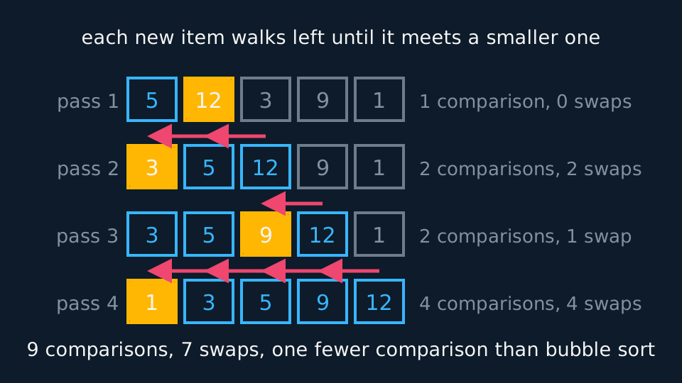
Shuttle sort builds the answer from the left instead. Take the items in turn, and move each one back through the part already sorted, swapping it with its left-hand neighbour while that neighbour is the larger and stopping the moment it is not. Pass 1 compares the first two items, pass 2 shuttles the third item back into place, and so on, so a list of n items takes n − 1 passes and the sorted part grows by one item each pass.
Describe the drawing
Four rows of five boxes, one row per pass. The first row is the list as it arrived, 5, 12, 3, 9, 1, since comparing the first two items finds them already in order. In each later row the item that has just been taken up is filled amber at the place it came to rest, and a coral arrow above the row marks every swap it made walking left. The boxes to the left of it are outlined in blue as the part now sorted, and that part grows by one box a pass until the last row reads 1, 3, 5, 9, 12. The counts down the right add to nine comparisons and seven swaps.
Quick sort picks a pivot and splits the list into those below it and those above it, keeping the original order within each part. The pivot is now fixed in place, and the method repeats on each sublist until every item has been a pivot. Which item serves as pivot is a convention rather than a rule, and the boards differ: this specification takes the middle item of each sublist, while others take the first value unless a question directs otherwise. Say which rule you are using, and hold to it in every sublist.
WORKED EXAMPLE
Three sorts on the same list
Sort 5, 12, 3, 9, 1 into increasing order by each method, counting the comparisons and the swaps as you go.
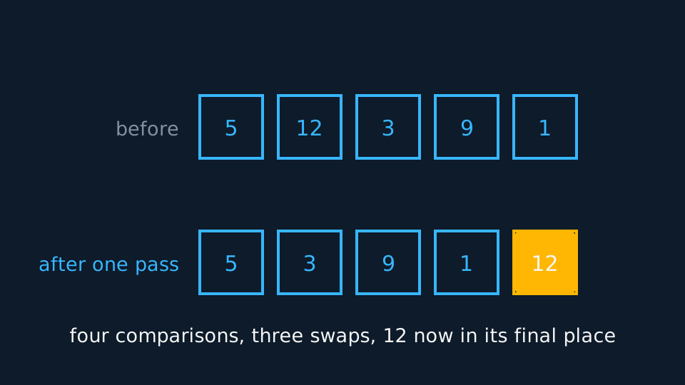
Bubble sort, first pass: compare and swap along the list to get 5, 3, 9, 1, 12, at a cost of 4 comparisons and 3 swaps. The largest is now in place.
Second pass: 3, 5, 1, 9, so 3 comparisons and 2 swaps. Third: 3, 1, 5, so 2 and 1. Fourth: 1, 3, so 1 and 1. A fifth pass makes no swaps, which is how the algorithm knows to stop.
That is 4 + 3 + 2 + 1 = 10 comparisons and 3 + 2 + 1 + 1 = 7 swaps.
Shuttle sort: pass 1 compares 5 and 12 and leaves them. Pass 2 shuttles 3 back past 12 and past 5, giving 3, 5, 12, 9, 1. Pass 3 takes 9 back past 12 and halts at 5. Pass 4 takes 1 back past 12, 9, 5 and 3.
That is 1 + 2 + 2 + 4 = 9 comparisons and 0 + 2 + 1 + 4 = 7 swaps: one comparison fewer than bubble sort, and the same number of swaps.
The swap counts agree for a reason. Both methods move items only by swapping neighbours, and one such swap repairs one out-of-order pair. This list holds seven of them, so seven swaps is what either method has to pay.
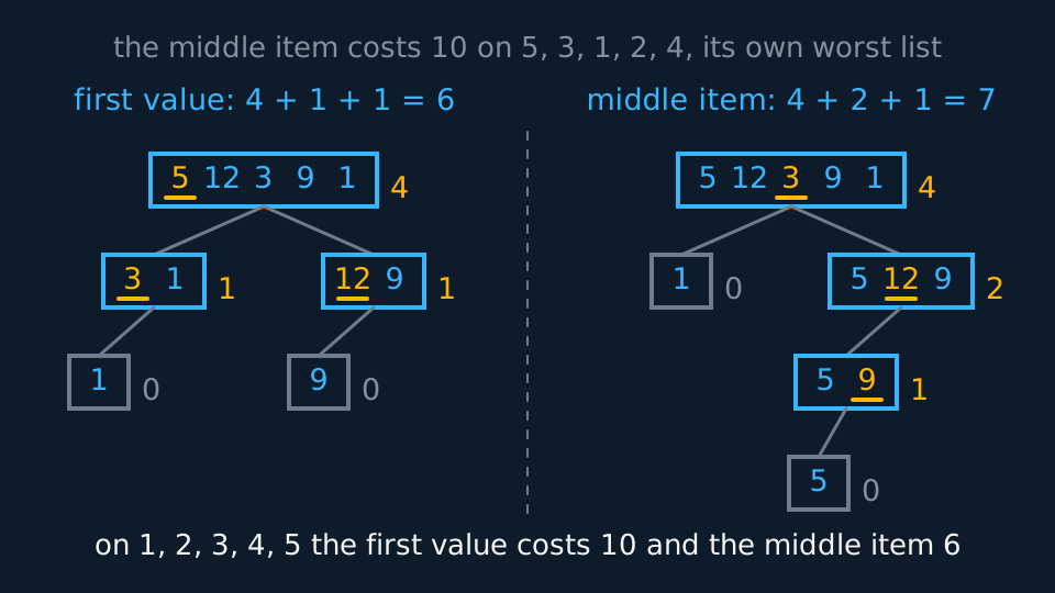
Quick sort takes the middle item, 3, as pivot. Comparing the other four items with it puts 1 on its left and 5, 12, 9 on its right, at a cost of 4 comparisons.
The sublist 5, 12, 9 has middle item 12, and two comparisons send 5 and 9 to its left. One more comparison orders those two, and each item has now served as a pivot.
That is 4 + 2 + 1 = 7 comparisons, and all three methods finish at 1, 3, 5, 9, 12. Pivoting on the first value instead would have cost 6 on this particular list.
The order of an algorithm
Counting comparisons on one list settles which method was quicker on that list and nothing further. To compare two methods before either is run, count on a list of n items instead. Write T(n) for the largest number of operations the method can need on a list of that length, which is its worst case time complexity.
Take bubble sort. Its first pass makes n − 1 comparisons, its second n − 2, and so on down to 1, so a run that goes the whole way makes (n − 1) + (n − 2) + ... + 1 comparisons. That is the sum of the first n − 1 positive integers, and since the first m positive integers add to m(m + 1)/2, it comes to n(n − 1)/2, which at n = 5 gives 10, the number counted above. The worst case is the input that forces the whole of it: a list in reverse order, where each comparison swaps as well.
The best case is a list already in order. The stopping rule then ends the method after one pass of n − 1 comparisons and no swaps, so bubble sort is linear on a sorted list and quadratic on a reversed one. A typical case sits between: about half the pairs of a randomly ordered list are out of order, so around n(n − 1)/4 swaps is what an average list costs, which is quadratic again. The three are different questions, and a question will say which of them it wants.
Order is what is left once everything that stops mattering is thrown away. Suppose a method needs T(n) = 2n3 + 50n2 + 300n + 1000 operations. The cubic term is 18 per cent of the total at n = 10 and 97.5 per cent at n = 1000. The dominant term, the one of highest power, is the part that survives, and its multiplier goes too, since doubling n multiplies any cubic term by 8 whatever sits in front of it. What is left is written O(n3).
Two methods labelled O(n2) and O(n3) can then be ranked without either being run, because the label is a statement about how the cost grows with the size of the problem rather than about one list. The powers wanted at this level are O(nk) with k = 0, 1, 2, 3 or 4, which read constant, linear, quadratic, cubic and quartic, and dominance is used in the informal sense above rather than defined.
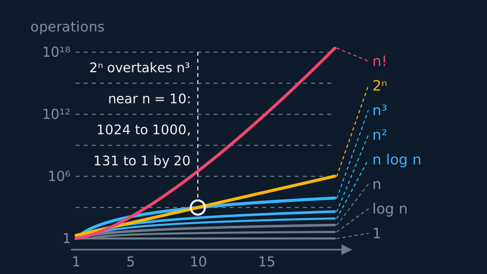
Three more orders sit outside that family, and where a formulae booklet prints the ranking it runs like this: O(1) is outgrown by O(log n), which is outgrown by O(n), then O(n log n), then O(n2), O(n3) and the higher powers, then O(an), the exponential orders, which outgrow every power once a is above 1, and last of all O(n!).
| Order | Cost at n = 10 | Cost at n = 20 | Where it turns up |
|---|---|---|---|
| O(1) | 1 | 1 | reading one entry of a matrix |
| O(log n) | 3.3 | 4.3 | halving a sorted list at each step |
| O(n) | 10 | 20 | one pass along a list |
| O(n log n) | 33 | 86 | the quickest sorting methods |
| O(n2) | 100 | 400 | bubble sort, shuttle sort, Dijkstra |
| O(n3) | 1000 | 8000 | Prim, Kruskal, Floyd |
| O(2n) | 1024 | 1 048 576 | trying every subset of the items |
| O(n!) | 3.6 × 10⁶ | 2.4 × 10¹⁸ | trying every tour of a network |
The last two rows are the reason large problems are handed to heuristics. At n = 10 the exponential row and the cubic row sit within 3 per cent of each other; at n = 20 the exponential row is 131 times the cubic one, and the factorial row is a number no machine will work through. That is why the travelling salesman problem is answered with bounds rather than by inspecting the tours.
Describe the drawing
Eight curves on one pair of axes, drawn against a vertical scale on which every gridline is a thousand times the one below it, so all eight fit for lists of up to twenty items. They leave the left-hand edge together and separate into a fan, and the name of each is written at the right-hand margin, reading downwards from n factorial through two to the n, the powers of n, n log n, n, log n and the constant. The exponential curve crosses the cubic one just short of n equal to ten, where the two costs are 1024 and 1000, and by twenty items it is 131 times the cubic and the factorial has left the page behind entirely.
Once the order is known, a run-time scales with it. A quadratic algorithm taking 0.5 seconds on a network of 20 nodes takes (100/20)2 = 25 times as long on one of 100 nodes, which is 12.5 seconds. A cubic one taking 0.4 seconds on 50 nodes takes 43 = 64 times as long on 200 nodes, which is 25.6 seconds. The orders needed for that scaling are stated in the lessons: Dijkstra is quadratic in the number of nodes, and Prim and Kruskal are cubic.
The two quick-sort pivot conventions build different recursion trees on the same five numbers, and the shape of the tree is where the count comes from: an even split costs less than a lopsided one.
Describe the drawing
Two recursion trees side by side, both starting from the list 5, 12, 3, 9, 1. Each box holds one sublist with its pivot underlined in amber, and the amber number beside the box is the comparisons that pivot costs. On the left the first value is taken each time and the tree splits evenly, four comparisons then one and one, six in all. On the right the middle item is taken, one sublist of three survives the first split, and the tree runs down one side for four, two and one, seven in all. Neither rule is the better one: on a list already in order the first value costs ten and the middle item six, and the middle item meets its own ten on 5, 3, 1, 2, 4.
WORKED EXAMPLE
The worst case for quick sort
Quick sort the list 1, 2, 3, 4, 5, pivoting on the first value of each sublist. Count the comparisons, give the order, and say whether the choice of pivot matters.
Pivot 1: four comparisons, and the other four items land to its right, so the sublist is 2, 3, 4, 5.
Pivot 2: three comparisons, leaving 3, 4, 5. Pivot 3: two comparisons. Pivot 4: one.
Total 4 + 3 + 2 + 1 = 10 comparisons, which is the same n(n − 1)/2 that bubble sort pays, so quick sort is O(n2) in the worst case.
A sorted list is the worst input for this pivot rule because the split is as lopsided as a split can be: one side of the pivot gets nothing, so the sublist shortens by one item at a time.
The middle-item rule halves this list at each step and costs only 6, so the choice of pivot certainly changes the work on a given list.
It does not change the worst-case order, though. Feed the middle-item rule the list 5, 3, 1, 2, 4 and its pivots come out 1, 2, 3, 4, splitting off nothing each time, for 10 comparisons again. A pivot rule chooses which input is its worst, not how bad that worst is, and quick sort is O(n2) either way.
Bin-packing algorithms and lower bounds
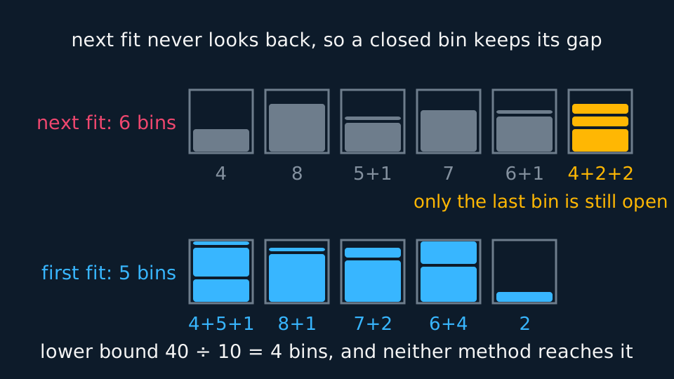
Bin packing puts items into bins of fixed size, and four methods are worth having. Next fit keeps one bin open: each item goes into it if there is room, and otherwise that bin is closed for good and a fresh one started. First fit takes the items in the order given and puts each into the first bin with room, going back to earlier bins to do it. That one difference, whether a bin may be reopened, costs next fit a whole extra bin on the ten items used below.
Describe the drawing
Two rows of open-topped bins of capacity ten, holding the same ten items in the same order. The upper row is next fit and needs six: the first bin takes the 4 and is then shut for good when the 8 arrives, so its gap of six is wasted, and five of the six bins are drawn grey to mark them closed. The lower row is first fit, which may return to any earlier bin and so fits the same items into five. Both are above the lower bound of four bins that the total of forty allows.
First fit decreasing sorts the items largest first, then packs by first fit. Full bin packing uses observation to spot groups of items that fill a bin exactly, packs those first, and finishes off whatever is left by first fit.
All four are heuristics, and they split in two on a second line. Next fit and first fit are online, deciding each item as it arrives and needing no sight of what is coming; first fit decreasing and full bin packing are offline, since one has to sort the list first and the other has to look it over. A question about items arriving one at a time on a conveyor is asking for an online method.
Next fit is the weakest of the four and the quickest, since it looks at one bin only. First fit decreasing is usually better than first fit and never much worse. Full bin is often better than both, but it needs a human eye and is hard to program.
The lower bound is the total of the items divided by the bin size, rounded up. Achieve it and the packing is certainly optimal and the question is finished. Miss it and the answer might still be optimal, but you would have to argue the point.
GUIDED PRACTICE
Packing by four methods
Pack the items 4, 8, 5, 1, 7, 6, 1, 4, 2, 2 into bins of size 10 by next fit, by first fit, by first fit decreasing and by full bin packing, and compare with the lower bound.
Show the working
Lower bound: the total is 40, so at least 40/10 = 4 bins.
Next fit gives (4), (8), (5, 1), (7), (6, 1), (4, 2, 2): 6 bins. The 4 and the 5 would have shared a bin, but by the time the 5 arrived the first bin had been closed.
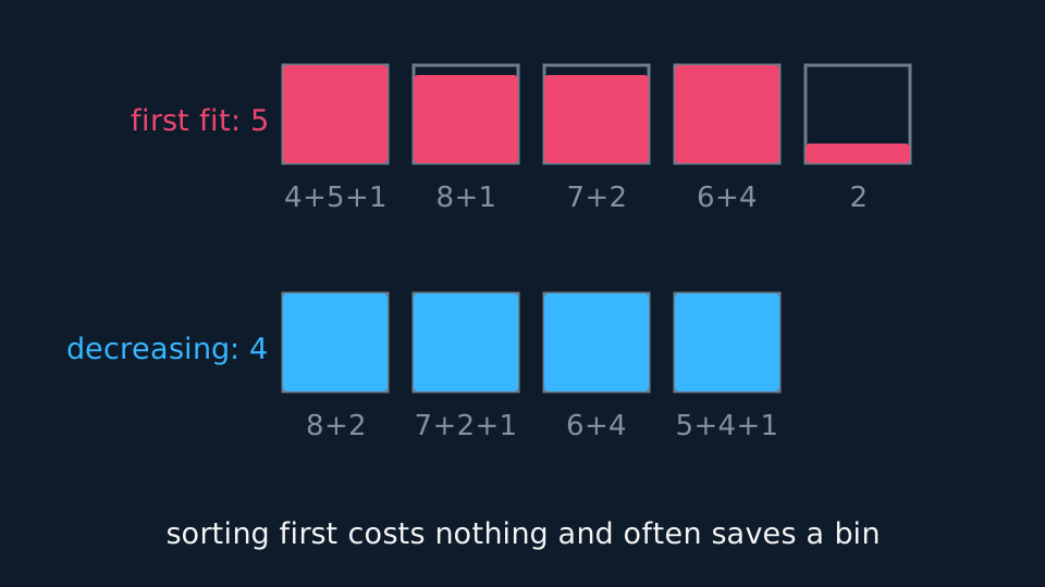
First fit gives (4, 5, 1), (8, 1), (7, 2), (6, 4), (2): 5 bins.
First fit decreasing gives (8, 2), (7, 2, 1), (6, 4), (5, 4, 1): 4 bins.
Full bins are easy to spot here: 8 + 2, 5 + 4 + 1, 7 + 2 + 1 and 6 + 4, again 4 bins and every one of them exactly full.
Two methods match the lower bound, so 4 bins is optimal and no further argument is needed.
ASSESSMENT FOCUS
- Asked to classify a problem, name the kind and say what its answer looks like: a yes or no with a reason, an object, a number, or a best object with a bound. A problem may fall into two kinds at once, since an optimisation question carries a construction inside it.
- Given pseudo-code, draw the trace table with one column per variable before running a single line.
- Show every pass of a sort as well as the final order, including the pass that ends a bubble sort by making no swaps.
- Bubble sort and shuttle sort both start at the left-hand end of the list unless the question says otherwise.
- For quick sort, say which pivot rule you are using: the middle item here, the first value on some papers, and whichever the question directs.
- Count comparisons and swaps separately. A question asking which method did less work names the operation it wants.
- Read the order off the dominant term and drop its multiplier, then say whether the count was a best, worst or typical case.
- Name which bin packing algorithm you are using and show the packing it produces, not only the number of bins.
- Asked whether a packing method suits items arriving one at a time, answer in the words online and offline.
- Compute the lower bound for a bin packing question and compare it with your packing.
CHECK YOURSELF
Items of size 6, 3, 5, 4, 2 are packed into bins of size 8. Find the lower bound and pack them by first fit decreasing.
Show a hint
Total over bin size, rounded up, then sort and pack.
Show the answer
Total 20, so the lower bound is 20/8 = 2.5, rounded up to 3 bins. Sorted: 6, 5, 4, 3, 2. First fit decreasing gives (6, 2), (5, 3), (4): 3 bins, which matches the bound.
An algorithm is a precise finite recipe, and its order says how the work grows with the size of the problem.
Count the operations on a list of n items, keep the dominant term and drop its multiplier: that is the order, written O(nk).
Next fit, first fit, first fit decreasing and full bin packing are all quick and none is guaranteed optimal.
Always compare a packing with the lower bound of total size over bin size, rounded up.
WORKBOOK
Printable practice for this topic: original exam-style questions with room to work, and a fully worked answer book. Free to use; please do not redistribute or sell.
Or read them with their worked answers on the algorithms, sorting and bin packing questions page.
USED LATER IN
CHECK YOUR PROGRESS
Rate how confident you feel with each objective for this lesson. Ratings are saved in this browser, on this device, unless you sign in.
- Sort a problem into the kinds existence, construction, enumeration and optimisation.
- Follow an algorithm given as text, as a flow chart or as pseudo-code, and record the trace.
- Use the INT and ABS functions inside an algorithm, and alter an algorithm to a new purpose.
- Perform bubble sort, shuttle sort and quick sort, showing every pass.
- Count the comparisons and the swaps two methods make on the same list.
- Write a worst-case run-time as a function of n, read its order off the dominant term, and rank the orders.
- Apply the four bin packing algorithms and compare the result with a lower bound.
- Say what makes a method an algorithm: an input, an output, determinism and termination.
Open the full revision checklist to see every objective in the course in one place.