Maths › Decision Mathematics 1 › Further packing and the knapsack problem
Further packing and the knapsack problem
Bin packing takes every item and asks for the fewest bins. The knapsack problem puts the opposite question to one container: with a limit on the mass it will carry and a profit attached to each item, which items are worth loading and which are left behind? Ranking by profit per kilogram and loading greedily is quick and can fall well short. Allowing fractions of an item bounds the best profit from above, a dynamic programming table settles the best load itself, and shelf packing carries the same questions into two dimensions.
Builds on Algorithms, sorting and bin packing and Simultaneous equations and inequalities.
IN THIS TOPIC
- Say what a knapsack problem asks for, and how the question it puts differs from a bin packing one.
- Write a knapsack problem as an integer programme with a nought-or-one variable for each item.
- Rank items by profit per unit mass, load greedily, and compare the result with the best load.
- Bound the best profit above by allowing fractions of items to be taken.
- Build the dynamic programming table and read the chosen items back out of it.
- Pack rectangles onto a sheet by shelves and compare the length used with the area lower bound.
- Stack boxes in a container by layers, and compare the height with the volume bound.
- Compare the cost of a complete search with the size of the table, and say what the unit of the limit does to it.
COMMON MISCONCEPTION
Loading the items with the greatest profit per kilogram first fills a knapsack for the greatest profit.
Loading by profit per kilogram is a heuristic, so treat its load as a candidate and check it. With crates of 3, 4, 5, 6 and 7 kg worth £24, £30, £36, £40 and £49 and a barrow carrying 10 kg, the density ranking loads the 3 kg and 4 kg crates for £54, while the 3 kg and 7 kg crates fill the barrow for £73. An exact answer needs the dynamic programming table.
The knapsack problem as an integer programme
Bin packing hands over the whole list of items and asks for the fewest bins. The knapsack problem puts a different question to a single container. Each item carries a mass and a profit, the container has a stated limit on the mass it will hold, and the load has to stay inside that limit while earning as much as it can. Items are left behind, and deciding which ones is the problem.
It is an optimisation question, and it has the shape a linear programme has: something to maximise, and a restriction that stops it running away. Writing it out in that shape before choosing a method fixes the objective and the constraint explicitly.
One instance runs through the first three sections. A stall holder has a barrow that carries 10 kg and five crates to choose between.
| Crate | Mass (kg) | Profit (£) | Profit per kg (£) |
|---|---|---|---|
| A | 3 | 24 | 8.00 |
| B | 4 | 30 | 7.50 |
| C | 5 | 36 | 7.20 |
| D | 6 | 40 | 6.67 |
| E | 7 | 49 | 7.00 |
Give crate i a variable xi that takes the value 1 when the crate is loaded and 0 when it is left on the ground. The whole problem then goes onto four lines.
| Part of the programme | Written out for these five crates |
|---|---|
| Variables | xi = 1 when crate i is loaded, xi = 0 when it is left, for i = 1 to 5 |
| Objective | maximise P = 24x1 + 30x2 + 36x3 + 40x4 + 49x5 |
| Constraint | 3x1 + 4x2 + 5x3 + 6x4 + 7x5 ≤ 10 |
| Integer condition | each xi takes the value 0 or 1 |
Every line but the last is linear, so this is a linear programme wearing one extra condition, and branch and bound, which this unit meets later, is one way at it. That last line is what makes the problem hard. With n items there are 2n subsets to choose between, which is 32 here and over a million at twenty items, so inspecting them all is an exponential method.
Loading by profit per kilogram
The greedy rule ranks the crates by profit per kilogram, which is also called the value density, and works down the ranking loading each crate that still fits. It costs one division per item and one sort, and it decides each crate without looking at what is left.
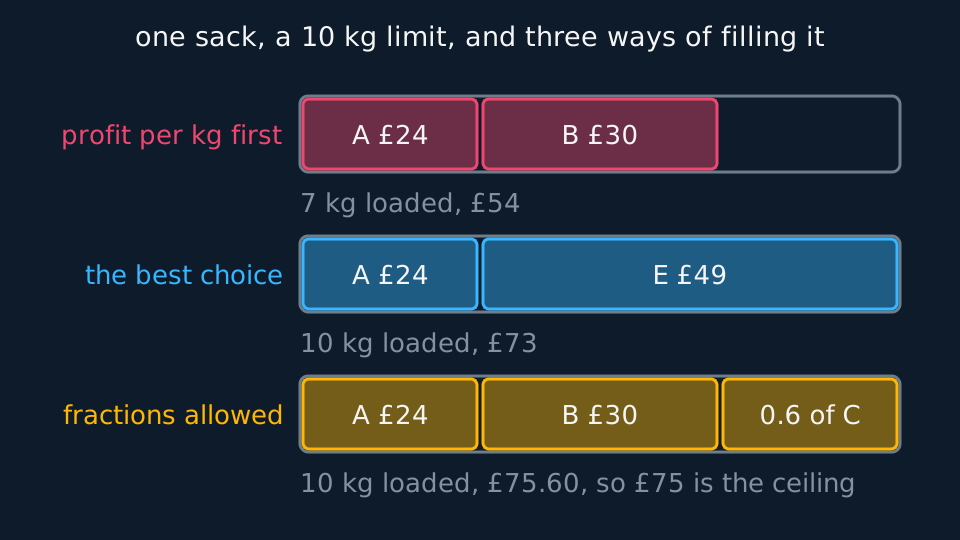
On these five the ranking is A at £8.00 per kg, B at £7.50, C at £7.20, E at £7.00 and D at £6.67. So A goes in, using 3 kg of the 10; B goes in, taking the load to 7 kg; and C, E and D each need more than the 3 kg still free. The barrow leaves with £54 aboard and 3 kg of room unused. It is not the best load.
WORKED EXAMPLE
The greedy load and the best load
Load the five crates above into a barrow carrying 10 kg by profit per kilogram, find the best load, and say what the greedy rule cost.
Ranking: A gives 24 ÷ 3 = 8.00, B gives 30 ÷ 4 = 7.50, C gives 36 ÷ 5 = 7.20, E gives 49 ÷ 7 = 7.00 and D gives 40 ÷ 6 = 6.67.
Greedy takes A, at 3 kg, then B, at 7 kg. C would carry the load to 12 kg, E to 14 kg and D to 13 kg, so none of the three fits. The load is A and B, worth £54.
Working through the subsets: A with E is 10 kg for £73, B with D is 10 kg for £70, B with C is 9 kg for £66, and nothing else reaches 70.
So the greedy rule fell £19 short, and the reason is visible in the masses. It spent 4 kg on B for £30, and those 4 kg were the room E needed. E alone is worth £49.
Swapping to another greedy rule is not a cure. Loading the most profitable crate first takes E and then A, which reaches £73 on this list and happens to be the best there is; on the list in the exercise below the same rule falls short. A heuristic that lands on the best answer for one instance has not been shown to be reliable, any more than first fit decreasing was by meeting the lower bound on one set of items.
An upper bound from fractional loading
The same ranking supplies a ceiling, and it costs nothing beyond the division already done. Drop the whole-crate condition, allow a crate to be split, and load in density order until the limit is reached. Splitting a crate widens the choice rather than narrowing it, so the fractional profit is at least the best whole-crate profit and is therefore an upper bound on it.
On the five crates: 3 kg of A at £24, then 4 kg of B at £30, then 3 of C's 5 kg, worth 3 × £7.20 = £21.60, for £75.60 in all. A whole-crate total is a whole number of pounds here, so the bound tightens to £75. Together with the greedy load of £54 that brackets the answer before any table is drawn, and the £2.60 between £73 and £75.60 is what the whole-crate condition costs.
Dynamic programming for the knapsack problem
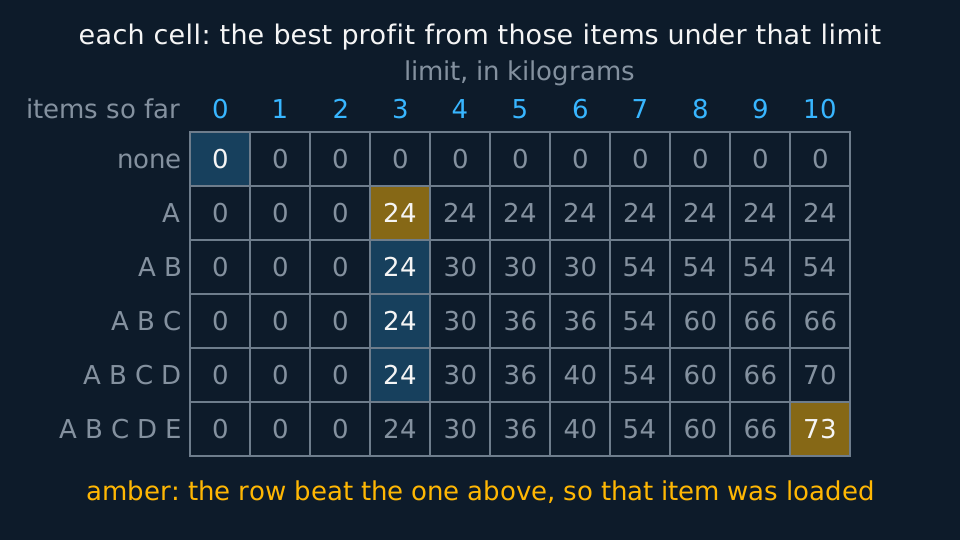
An exact answer needs a method that looks ahead, and the standard one is dynamic programming, worked here as a table. Write V(i, w) for the largest profit reachable from the first i crates alone under a limit of w kilograms. The table carries a row for each i and a column for each whole-number limit from 0 up to the real one.
One decision sits behind each cell. Crate i is either left, in which case the profit is V(i − 1, w), or loaded, which uses mi kilograms and pays pi, leaving V(i − 1, w − mi) to be earned from the crates before it. So V(i, w) is the larger of those two. Where mi is above w the second option is not open, and the cell copies the one above it.
The principle underneath that line is the one dynamic programming rests on. Whatever the best load does about crate i, what it does with the crates before i has to be the best use of the room they were left, or the load could be improved without touching crate i. That is why one comparison per cell is enough.
The top row is nought all the way across, since a choice made from no crates at all gives a profit of zero, and each later cell is one comparison away from cells already written down. Filling the rows in turn, left to right, completes the table with no searching at all.
WORKED EXAMPLE
Filling the table and reading the load back
Build the table for the five crates under a 10 kg limit, then name the crates in the best load.
Row A: a limit below 3 kg leaves the cell at 0, and from 3 kg upwards the cell is 24, since A is the only crate on offer.
Row B at a limit of 4: leaving B gives the 24 above it, loading B costs 4 kg and pays 30 with nothing left over, so the cell is 30 and the choice has changed which crate is aboard.
Row B at a limit of 7: leaving B gives 24, loading B pays 30 and leaves V(A, 3) = 24 behind it, for 54. The cell is 54.
Row E at the full 10: leaving E gives the 70 in the cell above, loading E costs 7 kg and pays 49 and leaves V(D, 3) = 24, for 73. The last cell is 73, which agrees with the search over the subsets.
Now read the load back by running up the last column. The 73 differs from the 70 above it, so E was loaded; take E's 7 kg off the limit and move to the column for 3 kg.
In that column the cells for D, C and B repeat the ones above them, so none of those was loaded. The cell for A holds 24 against the 0 above it, so A was loaded and the limit falls to 0.
The load is A and E, 10 kg, £73, which is the pair the subset search found and the pair the greedy rule missed.
The table here is 5 rows by 11 columns, so 55 cells against 32 subsets, and on a problem this small it saves nothing. The saving arrives with size, because the work goes as the number of items times the limit rather than as 2n: twenty crates under the same 10 kg limit need 220 cells where the subsets number 1 048 576. The catch is the limit itself. A barrow rated in grams has the same crates and a table a thousand times as wide, so the method is quick in the number of items and slow in the size of the limit.
GUIDED PRACTICE
A load neither greedy rule finds
A van carries 9 kg. The crates are J at 3 kg for £30, K at 4 kg for £34, L at 5 kg for £44 and M at 6 kg for £46. Load by profit per kilogram, then by profit, and then find the best load.
Show the working
Profit per kilogram: J gives £10.00, L gives £8.80, K gives £8.50 and M gives £7.67.
By that ranking J goes in at 3 kg and L takes the load to 8 kg. K would need 12 kg and M 14 kg, so the load is J and L, £74.
By profit the order is M, L, K, J. M goes in at 6 kg; L would take the load to 11 kg and K to 10 kg, so both are refused; J finishes the load at 9 kg. That is M and J, £76.
The subsets: K with L is 9 kg for £78, J with M is 9 kg for £76, J with L is 8 kg for £74, and no other pair fits.
So the best load holds neither the densest crate J nor the most profitable crate M. Neither greedy rule finds it, and a question asking for the best load wants the table.
Packing in two dimensions
Bin packing and the knapsack both run along one dimension: an item has a size, and sizes add. Cutting shapes from a sheet does not behave that way. A set of rectangles has to be laid on a roll of fixed width without overlapping and without being turned, and what has to be made small is the length of roll used. Two sets of the same total area can leave very different amounts of the roll unusable, so the sizes no longer simply add.
Shelf packing is the standard heuristic, and it turns the problem back into one dimension. Sort the rectangles by decreasing height. Lay them along the bottom of the roll, left to right, while the width allows; when the next one will not fit, close that shelf at the height of its tallest rectangle and start a fresh shelf on top. That is first fit decreasing with a second measurement attached, and it inherits the speed along with the weakness.
The bound comes from area rather than from length. The rectangles cover a fixed area, and the roll they lie on is a rectangle of known width, so the length used is at least the total area divided by the width. It is also at least the height of the tallest piece. Reach either figure and the packing is settled, in the same way a packing meeting the bin-packing lower bound finishes that question.
WORKED EXAMPLE
Six pieces on a sheet of width 12
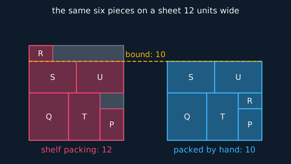
The pieces are P 3 by 4, Q 5 by 6, R 3 by 2, S 6 by 4, T 4 by 6 and U 6 by 4, width given first, and the sheet is 12 units wide. Pack them by shelves, compare the result with the area bound, and improve on it.
Sorted by decreasing height: Q and T at 6, then P, S and U at 4, then R at 2.
Shelf 1 takes Q at width 5, T at width 4 and P at width 3, which fill the 12; S would need 6 more. The shelf is 6 high, set by Q and T, so P leaves a gap 3 wide and 2 high above it.
Shelf 2 takes S and U, 6 and 6, filling the width again, and is 4 high. Shelf 3 holds R alone and is 2 high, wasting the other 9 units of its width. The height used is 6 + 4 + 2 = 12.
The area bound: the pieces cover 12 + 30 + 6 + 24 + 24 + 24 = 120 square units and the sheet is 12 wide, so no packing gets below 120 ÷ 12 = 10.
Move R into the gap above P and the third shelf disappears. Q, T and P along the bottom with R sitting on P fill a band 6 high; S and U fill a band 4 high above it; and the sheet stops at 10 with no waste at all.
That packing meets the bound, so 10 is optimal and the question is finished. The shelf rule lost 2 units because a shelf's height is fixed by its tallest piece and R arrived after the earlier shelves had closed.
Three dimensions changes the arithmetic and little else. Boxes go into a container, the heuristic fills one layer at a time, and the bound is the total volume divided by the area of the base.
ASSESSMENT FOCUS
- Say which rule you are loading by. Profit per kilogram and profit are different rules and give different loads.
- Divide profit by mass for every item before loading anything, and write the ranking out.
- Treat a greedy load as a candidate rather than as the answer: compare it with the subsets or with the table.
- Formulating a knapsack problem means a nought-or-one variable for each item, one objective, one mass constraint and the integer condition on its own line.
- Head the dynamic programming table with the items down the side and the limit across the top, and fill it a row at a time.
- Name the items in the load, not only the profit: run up the last column and note each place where the number rose.
- For a two-dimensional packing, sort by height, say where each shelf closes and why, and give the height of every shelf.
- Work out the area bound for a two-dimensional packing and compare it with the length you used, just as you would for bins.
CHECK YOURSELF
A rucksack carries 9 kg. The items are F at 3 kg for £18, G at 5 kg for £35 and H at 6 kg for £39. Load by profit per kilogram, and say whether that load is the best there is.
Show a hint
Divide profit by mass first, then look at what was left out.
Show the answer
Profit per kilogram: G £7.00, H £6.50, F £6.00. The rule loads G, passes over H because 11 kg is above the limit, then loads F, for 8 kg and £53. But H with F is 9 kg and £57, so the greedy load is not the best: G took the room that the heavier H needed.
A knapsack problem is an integer programme: a nought-or-one variable for each item, a profit to maximise and one mass constraint.
Loading by profit per unit mass is quick and can fall short, so treat the load it gives as a candidate and check it.
The table V(i, w), the best profit from the first i items under a limit of w, settles the answer, and running up its last column names the items.
In two dimensions pack by shelves of decreasing height and compare the length used with the total area divided by the width.
WORKBOOK
Printable practice for this topic: original exam-style questions with room to work, and a fully worked answer book. Free to use; please do not redistribute or sell.
Or read them with their worked answers on the further packing and the knapsack problem questions page.
CHECK YOUR PROGRESS
Rate how confident you feel with each objective for this lesson. Ratings are saved in this browser, on this device, unless you sign in.
- Say what a knapsack problem asks for, and how the question it puts differs from a bin packing one.
- Write a knapsack problem as an integer programme with a nought-or-one variable for each item.
- Rank items by profit per unit mass, load greedily, and compare the result with the best load.
- Bound the best profit above by allowing fractions of items to be taken.
- Build the dynamic programming table and read the chosen items back out of it.
- Pack rectangles onto a sheet by shelves and compare the length used with the area lower bound.
- Stack boxes in a container by layers, and compare the height with the volume bound.
- Compare the cost of a complete search with the size of the table, and say what the unit of the limit does to it.
Open the full revision checklist to see every objective in the course in one place.