Maths › Differential equations › Modelling with differential equations
Modelling with differential equations
Define the dependent and independent variables and the parameters, with their units, before forming the equation. State the modelling assumptions, solve the resulting differential equation, and interpret the solution only over the range where those assumptions are reasonable. Long-term behaviour follows from the particular integral only when the model is stable.
Builds on Second order equations and Forces and Newton's laws.
IN THIS TOPIC
- Recognise simple harmonic motion from its differential equation and state period and amplitude.
- Model a damped oscillator and interpret each term physically.
- Classify light, critical and heavy damping via the discriminant.
- Reduce a suitable linear coupled pair of first order equations to one second order equation.
- State the stability condition on the roots before reading a particular integral as the long-term behaviour.
COMMON MISCONCEPTION
Adding any amount of damping to an oscillator removes the oscillation entirely.
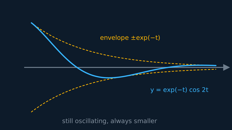
The discriminant decides. For y'' + by' + cy = 0 with b ≥ 0 and c > 0, b2 − 4c < 0 is light damping, which still oscillates, inside an envelope that decays. The oscillation stops only once b2 − 4c reaches 0 (critical damping) or exceeds it (heavy damping). y'' + 2y' + 5y = 0 has roots −1 ± 2i and the solution e−tcos 2t: frequency 2, with the amplitude decaying.
Simple harmonic motion
With resistance neglected, a mass on a spring obeys ẍ = −ω²x: the acceleration is proportional to the displacement and directed towards the equilibrium position. The auxiliary equation m² + ω² = 0 has roots ±ωi, so x = A cos ωt + B sin ωt. Written in harmonic form that is R cos(ωt − α), which shows the amplitude R = √(A² + B²) and the period 2π/ω at a glance. The initial displacement and velocity fix A and B, and with them the amplitude. Only the period 2π/ω is independent of where the mass started, and this is the property that makes a pendulum keep time, provided its swings stay small enough for the small-angle model behind ẍ = −ω²x.
Damping in three cases
After division by mass, a linear mass–spring–damper model has y″ + by′ + cy = f(t), with b ≥ 0 and c > 0: the y term is the restoring force per unit mass and the y′ term the resistance. For the unforced case f = 0, the discriminant of the auxiliary equation classifies the behaviour. b² − 4c < 0 is light damping: oscillation inside a decaying envelope. b² − 4c = 0 is critical damping, the fastest non-oscillatory return in this model, although for some initial conditions the solution crosses the equilibrium once. b² − 4c > 0 is heavy damping, a slower non-oscillatory return.
WORKED EXAMPLE
A lightly damped oscillator
Solve y'' + 2y' + 5y = 0 with y(0) = 1, y'(0) = −1.
The auxiliary equation m² + 2m + 5 = 0 has roots m = −1 ± 2i.
So y = e−t(A cos 2t + B sin 2t).
y(0) = 1 gives A = 1. Differentiating and setting y'(0) = −1 gives B = 0.
y = e−tcos 2t. Frequency 2 from the imaginary part, decay rate 1 from the real part.
With an external forcing term the equation is y'' + by' + cy = f(t). If the homogeneous roots have negative real parts, the complementary function tends to zero and the particular solution describes the persistent response. That interpretation requires that stability condition: if a root has non-negative real part, the complementary function does not tend to zero and the particular integral is not the long-term behaviour.
Coupled systems
Two connected tanks, or a similar pair of linked quantities, give a coupled pair in which dx/dt involves y and dy/dt involves x. A suitable linear coupled pair can be reduced to one second-order equation by differentiation and substitution; solve that equation, then recover the second variable from the first equation. Nonlinear systems, such as the predator-prey model with a product term xy, need not reduce in this way.
WORKED EXAMPLE
Reducing a linear coupled pair
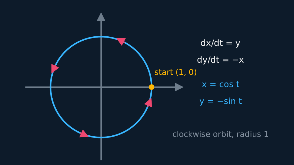
Solve dx/dt = y and dy/dt = −x with x(0) = 1, y(0) = 0.
Differentiating the first gives x'' = dy/dt = −x, so x'' + x = 0.
Auxiliary m² + 1 = 0 gives x = A cos t + B sin t.
x(0) = 1 gives A = 1. Since y = x' = −A sin t + B cos t, the condition y(0) = 0 gives B = 0.
x = cos t, y = −sin t. Since x² + y² = 1, the point (x, y) moves clockwise round the unit circle; both roots are purely imaginary, so the motion neither grows nor decays in this model.
INDEPENDENT PRACTICE
Reading the damping
A shock absorber obeys y'' + 6y' + 9y = 0. Classify the damping and give the general solution.
Show the working
The discriminant is 36 − 36 = 0, so the damping is critical.
Repeated root m = −3, so y = (A + Bt)e−3t.
Critical damping is a common design target for vehicle suspension, since it gives the fastest return to equilibrium without oscillation in this model.
ASSESSMENT FOCUS
- Define the variables and their units, and state the modelling assumptions, before forming the equation.
- Interpret the constants in context: after division by mass, the y' coefficient is the resistance per unit mass and the y coefficient the stiffness per unit mass, with b ≥ 0 and c > 0.
- Quote the value of the discriminant when classifying damping.
- For SHM, read ω from the equation and give the period as 2π/ω.
- In a coupled system, state which equation is differentiated and where the substitution is made, and check that the system is linear.
- Recover the second variable from one of the original first order equations.
- State the stability condition before describing a particular integral as the long-term behaviour.
CHECK YOURSELF
Classify the damping in y'' + 6y' + 9y = 0 and state the long-term behaviour of any solution.
Show a hint
Compute b² − 4c and look for a repeated root.
Show the answer
36 − 36 = 0, so the damping is critical. The repeated root m = −3 gives y = (A + Bt)e−3t. The root has negative real part, so every solution tends to zero without oscillating.
SHM is ẍ = −ω²x, with period 2π/ω and amplitude determined by the initial conditions.
For y″ + by′ + cy = 0 with b ≥ 0 and c > 0, the sign of b² − 4c classifies the damping: negative gives oscillation inside a decaying envelope, zero critical damping, positive heavy damping.
A suitable linear coupled pair reduces to one second order equation by differentiating one equation and substituting the other; nonlinear systems need not reduce this way.
WORKBOOK
Printable practice for this topic: original exam-style questions with room to work, and a fully worked answer book. Free to use; please do not redistribute or sell.
Or read them with their worked answers on the modelling with differential equations questions page.
CHECK YOUR PROGRESS
Rate how confident you feel with each objective for this lesson. Ratings are saved in this browser, on this device, unless you sign in.
- Recognise simple harmonic motion from its differential equation and state period and amplitude.
- Model a damped oscillator and interpret each term physically.
- Classify light, critical and heavy damping via the discriminant.
- Reduce a suitable linear coupled pair of first order equations to one second order equation.
- State the stability condition on the roots before reading a particular integral as the long-term behaviour.
Open the full revision checklist to see every objective in the course in one place.