Maths › Further Statistics 1 › Type I and Type II errors, test size and power
Type I and Type II errors, test size and power
Test size is the probability of a Type I error. Power is the probability of rejecting the null hypothesis when a specified alternative is true. Calculate both from a critical region, evaluate a power function, and state how size and power move together when the critical region changes.
Builds on Hypothesis tests for Poisson and geometric models and Hypothesis testing with the binomial.
IN THIS TOPIC
- Distinguish Type I and Type II errors and compute their probabilities.
- Find the size of a test from its critical region.
- Evaluate and interpret the power function at particular alternatives.
COMMON MISCONCEPTION
A test at the 5% level is wrong 5% of the time.
The 5% is the probability of rejecting H₀ when H₀ is true, which is the size of the test, and for a discrete statistic the size usually falls a little below that nominal level. It says nothing about the other failure, a Type II error, whose probability depends on which alternative is true; the power at an alternative is 1 minus that probability.
Type I and Type II errors
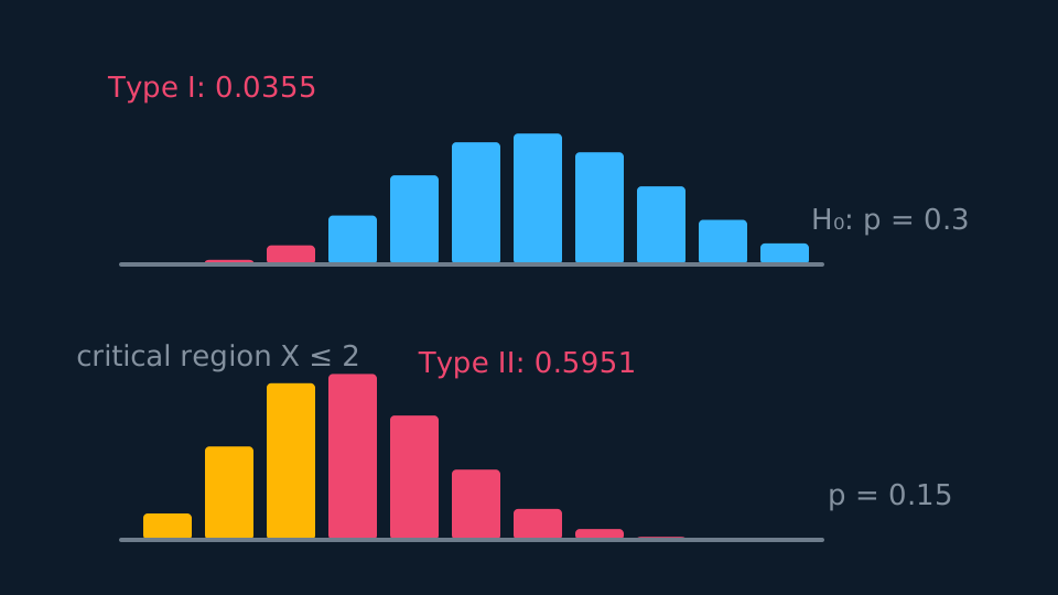
A Type I error rejects a true H₀, which is a false alarm. Its probability is the size of the test, meaning the actual probability of landing in the critical region when H₀ holds. For a discrete distribution that usually falls a little below the nominal level. A Type II error fails to reject H₀ when some alternative is true, which is a miss.
The 5% figure describes only the first kind of failure, and only in the world where H₀ is true. Reading it as an overall error rate mistakes a conditional probability for an unconditional one, and ignores Type II errors entirely.
Describe the drawing
Two binomial bar charts stacked. In the upper one, for the null value of p, the three bars inside the critical region are coral: their total is the Type I risk. In the lower one, for an alternative p of nought point one five, the coral bars are those outside the region: their total is the chance of missing the change.
WORKED EXAMPLE
Size and Type II probability
For X ~ B(20, p), H₀: p = 0.3 against H₁: p < 0.3, with critical region X ≤ 2. Find the size, and the probability of a Type II error when p = 0.15.
Size = P(X ≤ 2 | p = 0.3) = 0.0355, below the nominal 5%, because adding X = 3 to the region would take it above 5%.
When p = 0.15: P(X ≤ 2) = 0.4049, so the test rejects with probability 0.4049.
The Type II probability is 1 − 0.4049 = 0.5951. This test misses a drop to 0.15 more often than it catches it.
The power function
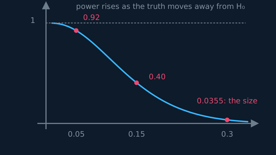
The power at a particular alternative is the probability of correctly rejecting H₀ there, so power equals 1 − P(Type II error). Plot it against the parameter and you have the power function. It sits low near H₀, where the truth is hard to tell apart from the null, and it rises towards 1 as the alternative moves further away.
WORKED EXAMPLE
Reading the power function
For the test above, the power is 0.0355 at p = 0.3, 0.2061 at p = 0.2, 0.4049 at p = 0.15 and 0.9245 at p = 0.05. Comment.
At p = 0.3 the power equals the size, as it must. H₀ is true there, so a 'correct rejection' is really a false alarm.
Detection improves steadily as p falls. Even at p = 0.15, though, nearly six departures in ten go unnoticed.
Only for large drops does the test become reliable. For a fixed test statistic and sample size, enlarging the critical region increases both the size and the power, so neither risk can be reduced without raising the other.
GUIDED PRACTICE
Comparing two tests
Test A has size 0.05 and power 0.62 at a given alternative; test B has size 0.01 and power 0.44 at the same alternative. Which is preferable, and on what grounds?
Show the working
Neither dominates. A detects the alternative more often, B raises fewer false alarms.
The choice depends on the costs. Where a missed change is expensive, prefer A. Where a false alarm triggers something costly, prefer B.
A larger sample often allows greater power at the same significance level; a more informative design or test statistic can also improve performance.
Choosing a significance level in context
Some questions ask for an argued choice of level rather than the application of a stated one. A screening test that misses a disease costs a patient more than a false positive costs the clinic, so a larger size may be accepted in return for greater power. A test that shuts down a production line whenever it rejects H₀ needs a small size.
In an answer, name what each error would mean in the situation described, state which consequence is more serious, and say which way that pushes the significance level.
ASSESSMENT FOCUS
- Compute the size from the critical region, not from the nominal level. For discrete tests the two differ.
- Type II probabilities need a specific alternative value. Without one the question is incomplete.
- Power = 1 − P(Type II error), evaluated at the stated alternative.
- When comparing tests, mention both size and power. Neither number judges a test on its own.
CHECK YOURSELF
A test has size 0.043 and, at a particular alternative, a probability of 0.68 of failing to reject H₀. State the probability of a Type I error and the power at that alternative.
Show a hint
Size is the Type I probability; power is one minus the Type II probability.
Show the answer
P(Type I error) = 0.043. Power = 1 − 0.68 = 0.32, so this test misses the alternative about two thirds of the time.
Type I rejects a true H₀, with probability equal to the test's size; Type II misses a real change.
Power = 1 − P(Type II error), rising as the alternative moves away from H₀, and with n fixed size and power trade off.
WORKBOOK
Printable practice for this topic: original exam-style questions with room to work, and a fully worked answer book. Free to use; please do not redistribute or sell.
Or read them with their worked answers on the Type I and Type II errors, test size and power questions page.
CHECK YOUR PROGRESS
Rate how confident you feel with each objective for this lesson. Ratings are saved in this browser, on this device, unless you sign in.
- Distinguish Type I and Type II errors and compute their probabilities.
- Find the size of a test from its critical region.
- Evaluate and interpret the power function at particular alternatives.
Open the full revision checklist to see every objective in the course in one place.