Maths › Statistics › Hypothesis testing with the binomial
Hypothesis testing with the binomial
A hypothesis test assesses a claim about a population proportion by calculating how unlikely the observed data would be if the claim were true. State the hypotheses, carry out one- and two-tailed binomial tests at a stated significance level, and find critical regions and actual significance levels.
Builds on The binomial distribution.
IN THIS TOPIC
- Set up H₀ and H₁ for a claim about a binomial probability p.
- Carry out one- and two-tailed tests by comparing a tail probability with the significance level, concluding in context.
- Find a critical region and state the actual significance level of a test.
COMMON MISCONCEPTION
Rejecting the null hypothesis proves the alternative is true.
A test rejects H₀ or does not reject it, and proves neither hypothesis. Everything is computed assuming H₀ is true, so rejection says only that data at least as extreme as those observed are less likely than the significance level under that assumption. Rejecting H₀ when H₀ is true has a probability of its own, the actual significance level of the critical region.
The logic of a test
The null hypothesis H₀ is the specified population claim being tested, always a particular value of the population proportion p. The alternative H₁ states the departure under investigation: p > 0.5 or p < 0.5 for a one-tailed test, p ≠ 0.5 for a two-tailed test. The significance level, usually 5%, is fixed before the data are collected and sets how unlikely the data must be for H₀ to be rejected. A test either rejects H₀ or does not reject it; it does not prove either hypothesis true.
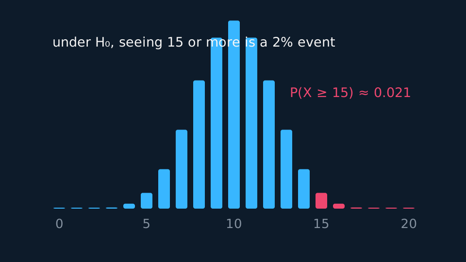
Everything is computed assuming H₀ is true: under H₀ the count follows a known binomial, so the probability of a result at least as extreme as the one observed, the p-value, can be found on a calculator.
A p-value is not the probability that H₀ is true, and it is not the probability that the result occurred by chance. It is the probability of data at least as extreme as those observed given that H₀ holds.
A one-tailed test
WORKED EXAMPLE
Is the coin biased towards heads?
A coin is flipped 20 times and lands heads 15 times. Test at the 5% level whether the coin is biased towards heads.
H₀: p = 0.5, H₁: p > 0.5. Under H₀, X ~ B(20, 0.5).
P(X ≥ 15) = 1 − P(X ≤ 14) = 0.0207.
0.0207 < 0.05, so at the 5% significance level reject H₀ and conclude that there is sufficient evidence that the coin is biased towards heads.
A complete conclusion has three parts: the comparison, the decision about H₀, and the interpretation in context.
The tail probability is P(X ≥ 15), not P(X = 15). The test uses the probability of a result at least as extreme as the one observed, and using the probability of the exact observed value can reverse the decision.
Two tails
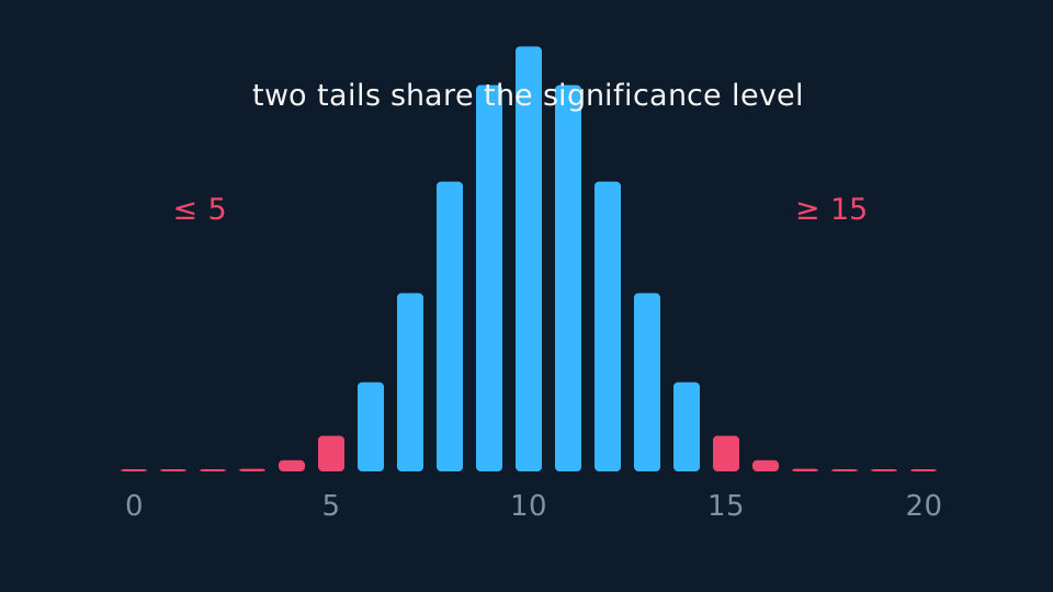
A two-tailed test splits the significance level between the two tails, 2.5% each at the 5% level, and the observed tail probability is compared with that half. The wording determines which test applies: “has the proportion changed” is two-tailed, “has it increased” is one-tailed.
WORKED EXAMPLE
A spinner that lands red too rarely
A spinner is claimed to land on red 30% of the time. In 25 spins it lands red 3 times. Test at the 5% level whether the proportion differs from 0.3.
H₀: p = 0.3, H₁: p ≠ 0.3. Under H₀, X ~ B(25, 0.3).
3 is below the expected 7.5, so this is the lower tail: P(X ≤ 3) = 0.0332.
Compare with 0.025, not with 0.05. Since 0.0332 > 0.025, at the 5% significance level do not reject H₀; there is insufficient evidence that the proportion of reds differs from 0.3.
Comparing 0.0332 with 0.05 instead would reverse the decision. In a two-tailed test the comparison is always against half the significance level.
Critical regions
Describe the drawing
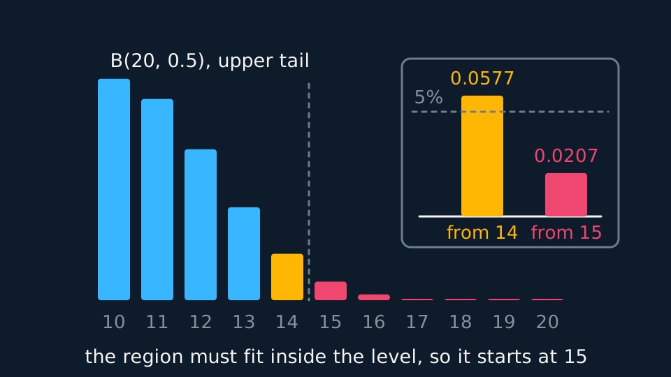
Bars of B(20, 0.5) from ten to twenty successes, the bar at fourteen amber and the bars from fifteen up coral, with an inset comparing the two candidate tail totals against a dashed five percent line: the tail from fourteen, 0.0577, pokes above the line and the tail from fifteen, 0.0207, stays below it, so the critical region is X at least fifteen.
A critical region is the set of values of the test statistic that lead to rejection of H₀, determined before the data are collected. For X ~ B(20, 0.5) against p > 0.5 at 5%, P(X ≥ 14) = 0.0577 exceeds 0.05 and P(X ≥ 15) = 0.0207 does not, so the critical region is X ≥ 15.
The actual significance level is the probability of the critical region under H₀, here 2.07%. Because the binomial takes only whole-number values, this probability is usually less than the nominal 5%. State its value and its meaning: it is the probability of rejecting H₀ when H₀ is true.
A two-tailed critical region is built one tail at a time, each against 2.5%. With X ~ B(25, 0.3), the region is X ≤ 2 or X ≥ 13, and its actual significance level is 0.00896 + 0.01747 = 0.02643, or 2.64%.
ASSESSMENT FOCUS
- State the hypotheses in terms of p: write “H₀: p = 0.3” rather than “the coin is fair”.
- Either compare a tail probability with the significance level or compare the observed value with a critical region, and state which method is being used.
- Write the conclusion in one of two forms: “At the stated significance level, reject H₀ and conclude that there is sufficient evidence of …”, or “At the stated significance level, do not reject H₀. There is insufficient evidence of …”, naming the context in each case.
- For a two-tailed test, halve the significance level before comparing.
- The actual significance level is the probability of the critical region under H₀, and is usually smaller than the nominal level.
- Do not use P(X = observed). The test uses the probability of a result at least as extreme, which is a tail probability.
CHECK YOURSELF
X ~ B(30, 0.2) under H₀, and the critical region for a one-tailed test is X ≥ 11 with P(X ≥ 11) = 0.0256. State the actual significance level and what it measures.
Show a hint
The region's probability, assuming the null.
Show the answer
The actual significance level is 2.56%.
It is the probability of rejecting H₀ when H₀ is true.
Assume H₀, calculate how extreme the data are under it, and compare with the stated significance level; then reject H₀ or do not reject it.
The critical region is decided before the data, and its probability under H₀ is the actual significance level.
WORKBOOK
Printable practice for this topic: original exam-style questions with room to work, and a fully worked answer book. Free to use; please do not redistribute or sell.
Or read them with their worked answers on the hypothesis testing with the binomial questions page.
USED LATER IN
CHECK YOUR PROGRESS
Rate how confident you feel with each objective for this lesson. Ratings are saved in this browser, on this device, unless you sign in.
- Set up H₀ and H₁ for a claim about a binomial probability p.
- Carry out one- and two-tailed tests by comparing a tail probability with the significance level, concluding in context.
- Find a critical region and state the actual significance level of a test.
Open the full revision checklist to see every objective in the course in one place.