Maths › Further Statistics 1 › Hypothesis tests for Poisson and geometric models
Hypothesis tests for Poisson and geometric models
The hypothesis-testing procedure carries over unchanged to Poisson and geometric models. Hypotheses are stated about the parameter, the tail probability of the observed result is computed, and that probability is compared with the significance level.
Builds on Geometric and negative binomial distributions and Hypothesis testing with the binomial.
IN THIS TOPIC
- State hypotheses about λ for a Poisson model or p for a geometric one.
- Find the tail probability of the observed value and compare with the level.
- Locate a critical region, find its actual size, and report conclusions in context.
COMMON MISCONCEPTION
Because the Poisson distribution has no fixed number of trials, hypothesis testing cannot be applied to it.
Nothing in the method needs a fixed number of trials. The hypotheses name the parameter, H₀: λ = λ₀ against a one- or two-tailed alternative, and the test compares the probability of a result at least as extreme as the one observed, computed assuming H₀ holds, with the significance level. Discreteness then puts the actual significance level below the nominal one.
Testing a rate
A Poisson test asks whether the underlying rate has changed. The hypotheses name the parameter, never the data. Write H₀: λ = λ₀ against a one- or two-tailed alternative. Nothing in the method needs a fixed number of trials. Compute the probability of a result at least as extreme as the one observed, assuming H₀ is true, and compare that with the significance level.
Be careful what you claim for that tail probability. It is the chance of data this extreme given that H₀ holds. It is not the probability that H₀ is true, and 1 minus it is not the probability that H₁ is true. A 5% level fixes how often the test raises a false alarm when the rate has not moved, and says nothing about how often it will notice a rate that has.
WORKED EXAMPLE
A rate under suspicion
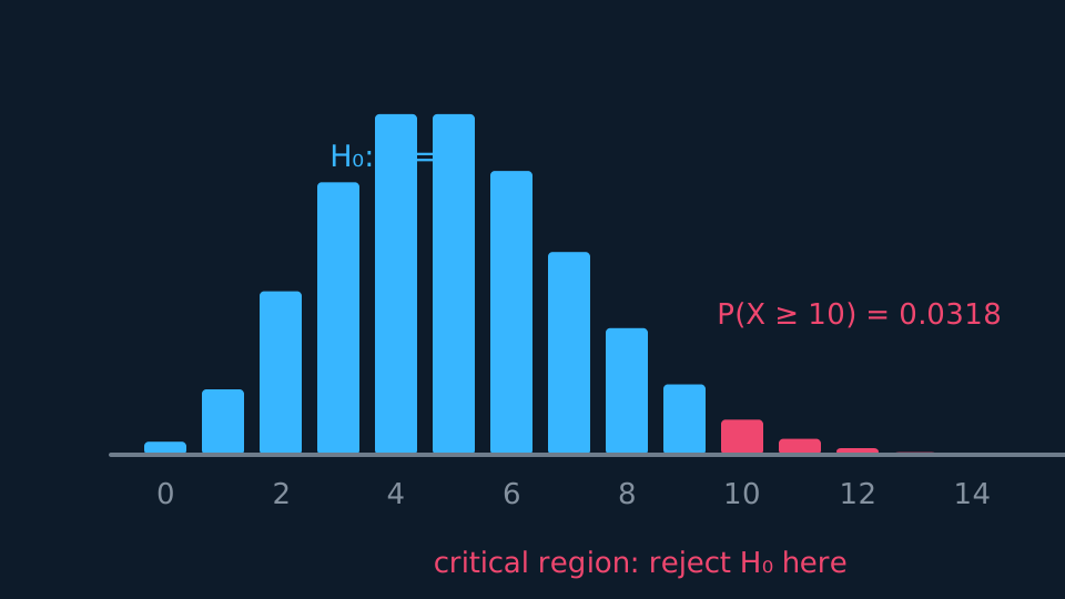
Complaints arrive at a mean of 5 per week. After a change of policy, 10 arrive in a week. Test at the 5% level whether the rate has increased.
H₀: λ = 5, H₁: λ > 5, one-tailed at 5%.
Assuming H₀, P(X ≥ 10) = 1 − P(X ≤ 9) = 0.0318.
0.0318 < 0.05, so reject H₀. There is evidence at the 5% level that the complaint rate has risen.
Finding the critical region
Some questions ask for the region before any data arrives. Work outwards from the tail until the accumulated probability first exceeds the level, then step back one. For the complaints above, P(X ≥ 9) = 0.0681 sits above 5% while P(X ≥ 10) = 0.0318 sits below, so the critical region is X ≥ 10.
Because the count is discrete, no region lands exactly on 5%. The actual significance level here is 0.0318, which is the probability of the critical region rather than the nominal 0.05. Two-tailed tests split the level, so each tail is built to at most half of it, and the two actual tail probabilities are added at the end.
WORKED EXAMPLE
A two-tailed critical region
Faults occur at Po(6) per shift. Find the critical region for a two-tailed test at the 5% level, and state the actual significance level.
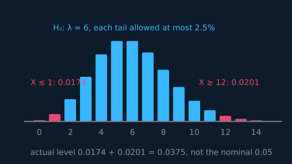
Each tail gets at most 2.5%. Lower tail: P(X ≤ 1) = 0.0174 and P(X ≤ 2) = 0.0620, so the lower region is X ≤ 1.
Upper tail: P(X ≥ 12) = 0.0201 and P(X ≥ 11) = 0.0426, so the upper region is X ≥ 12.
The critical region is X ≤ 1 or X ≥ 12, with actual significance level 0.0174 + 0.0201 = 0.0375.
Describe the drawing
A Poisson bar chart for a mean of six with both ends shaded coral: the bars at nought and one, holding nought point nought one seven four together, and the bars from twelve upwards, holding nought point nought two nought one. Each tail is the widest that stays inside its two and a half per cent, one more bar on either side would break it, and the actual significance level is the sum nought point nought three seven five rather than the nominal five per cent.
Testing a waiting time
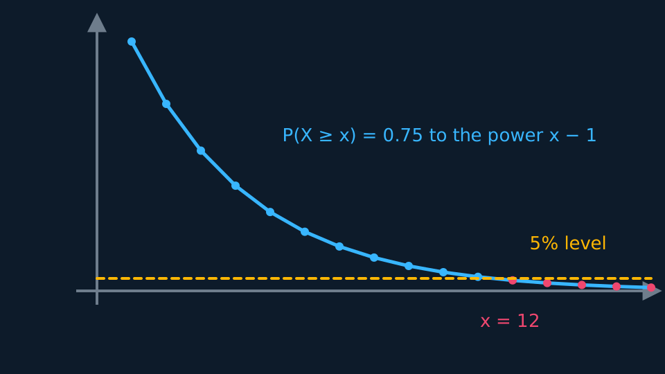
For a geometric model the parameter is p, and a long wait is evidence that p is smaller than claimed. The upper tail has a closed form: needing at least x trials means the first x − 1 all failed, so P(X ≥ x) = (1 − p)x-1 exactly, and no summation is required.
WORKED EXAMPLE
A machine that keeps missing
A process is claimed to succeed with probability 0.25 per attempt. The first success comes on the 12th attempt. Test at the 5% level whether p is smaller than claimed.
H₀: p = 0.25, H₁: p < 0.25. A small p means a long wait, so the evidence sits in the upper tail of X.
P(X ≥ 12) = 0.75¹¹ = 0.0422.
0.0422 < 0.05, so reject H₀. There is evidence that the success probability is below 0.25.
GUIDED PRACTICE
A two-tailed Poisson test
Faults occur at Po(8) per shift. A new shift records 3 faults. Test at the 5% level whether the rate has changed.
Show the working
H₀: λ = 8, H₁: λ ≠ 8, two-tailed, so each tail carries 2.5%.
The observed value is low, so compute the lower tail: P(X ≤ 3) = 0.0424.
0.0424 > 0.025, so do not reject H₀. There is insufficient evidence at the 5% level that the fault rate has changed. Halving the level for a two-tailed test is what changes the verdict here.
ASSESSMENT FOCUS
- State hypotheses in terms of λ or p, never in terms of the sample value.
- Halve the significance level for each tail of a two-tailed test, and say on the page that you have.
- For geometric upper tails use (1 − p) to the power x − 1 instead of summing terms.
- Actual significance level means the probability of the critical region you found, not the nominal 5%.
- Finish in context by naming the rate or the process: 'reject H₀' alone does not state a conclusion about the situation described.
CHECK YOURSELF
For a Poisson model with H₀: λ = 4 and H₁: λ > 4, the observed value is 9 and P(X ≥ 9) = 0.0214. State the conclusion at the 5% level.
Show a hint
Compare the tail probability with 0.05.
Show the answer
0.0214 < 0.05, so reject H₀. There is evidence at the 5% level that the mean rate has increased above 4.
Poisson tests fix hypotheses on λ, and you compare the tail probability of the observed count under H₀ with the level.
Discreteness drops the actual significance level below the nominal one, and geometric upper tails are (1 − p) to the power x − 1.
WORKBOOK
Printable practice for this topic: original exam-style questions with room to work, and a fully worked answer book. Free to use; please do not redistribute or sell.
Or read them with their worked answers on the hypothesis tests for Poisson and geometric models questions page.
CHECK YOUR PROGRESS
Rate how confident you feel with each objective for this lesson. Ratings are saved in this browser, on this device, unless you sign in.
- State hypotheses about λ for a Poisson model or p for a geometric one.
- Find the tail probability of the observed value and compare with the level.
- Locate a critical region, find its actual size, and report conclusions in context.
Open the full revision checklist to see every objective in the course in one place.