Physics › Required practicals › Charging and discharging a capacitor
REQUIRED PRACTICAL 9Charging and discharging a capacitor
Following the charge and discharge of a capacitor, and using a log-linear plot to determine the time constant RC.
Theory: Charging and discharging · The time constant and exponential decay
What you are trying to do
Follow the pd across a capacitor with a voltmeter and stopclock as it discharges through a resistor, then as it charges through one, and use log-linear plots to find the time constant RC, and from it the capacitance.
Apparatus
- A large-value capacitor, for example 470 μF (note its polarity if it is electrolytic)
- A resistor chosen to make RC tens of seconds, for example 100 kΩ
- A 6 V battery pack and a two-way switch, with a series resistor in the charging path where the capacitor, switch or supply ratings call for one
- A digital voltmeter of high input resistance, connected across the capacitor
- A stopclock, or a data logger with a voltage sensor in place of the stopclock and voltmeter
Variables
- Independent: time since the discharge began
- Dependent: the pd across the capacitor
- Control: the resistance, the capacitance and the starting pd: the same components and the same fully charged start each run
Method
- Choose components so the time constant suits a stopclock: 100 kΩ with 470 μF gives RC of 47 s, slow enough to read by eye. A small RC would be over before your first reading.
- Charge the capacitor by moving the switch to the battery side, and wait until the voltmeter has settled at the full 6.0 V. Include suitable current limiting where required by the capacitor, switch and supply ratings; do not deliberately short a capacitor across a low-resistance source.
- Flick the switch to the discharge side and start the clock at the same instant; this synchronisation is the single biggest source of timing error, so practise the flick-and-start before recording.
- Read the pd at fixed intervals, every ten seconds here, until it has fallen to well under half its starting value. Repeat the whole run at least twice and average the readings at each time.
- The activity is charging and discharging, so do the other half too: move the resistor into the battery side of the switch so the capacitor charges through it, start from a fully discharged capacitor, and log the rising pd at the same fixed intervals. It climbs towards the supply value with the same time constant RC.
Analysis
- The model to test is exponential decay, . Taking logarithms straightens it. A logarithm takes a pure number, so divide each pd by a fixed reference pd before taking it. With a reference of 1 V, the quantity plotted is ln(V / 1 V), and the model gives ln(V / 1 V) = ln(V0 / 1 V) − t/RC, a straight line in t. That is what the column heading ln (V / V) records: the logarithm of a ratio, not of a pd.
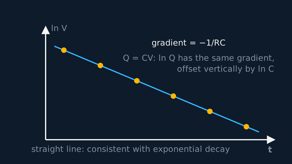
Describe the drawing
Six amber data points lying exactly on a straight falling line of the natural log of the p.d. against time: the log-linear plot from required practical nine, whose gradient hands you minus one over RC. Because the charge is C times the p.d., plotting ln Q instead gives a parallel line with the very same gradient, offset vertically by the constant ln C.
- Plot ln(V / 1 V) against t. A straight line is consistent with the exponential over the range measured; a clear curve would refute it. The gradient equals −1/RC, so RC is minus one over the gradient. Changing the reference pd moves the intercept and leaves the gradient alone.
- Divide RC by the known resistance to obtain the capacitance, and compare with the value printed on the component.
- The charging data get the same treatment with one change. The pd obeys , so it is the shortfall from the final value, V0 − V, that decays exponentially: plot ln((V0 − V) / 1 V) against t, and a straight line of gradient −1/RC should return the same time constant as the discharge run.
- What the straight log line establishes. It is a stronger statement than a falling pd. It says the data are consistent with exponential decay across the range measured, the fractional loss per second holding constant there, which supports the model without ruling out every alternative outside that range. The gradient gives RC of about 47 s, and dividing by the resistor gives a capacitance within a few per cent of the marked 470 μF. That agreement shows the capacitor is within its quoted tolerance. It does not establish that your value is the more accurate of the two: a tightly fitted line is precise, and its accuracy still depends on the resistor's own tolerance, on the voltmeter's loading and on the timing.
- What a stopclock cannot follow. The first second of the discharge is gone before you can read anything, so the steepest part of the curve is never sampled and the exponential is tested over the part of its range that changes slowly. Choosing RC in tens of seconds is what makes the experiment possible at all, and it is also what leaves that hole. A data logger taking ten readings a second closes it, and lets you use a smaller RC where the voltmeter's own leakage path matters less.
A worked set of readings
One discharge run with the circuit above, read every ten seconds:
| t / s | V / V | ln (V / V) |
|---|---|---|
| 0 | 6.00 | 1.792 |
| 10 | 4.85 | 1.579 |
| 20 | 3.92 | 1.366 |
| 30 | 3.17 | 1.153 |
| 40 | 2.56 | 0.941 |
| 50 | 2.07 | 0.728 |
| 60 | 1.67 | 0.515 |
Idealised illustrative data, chosen so the working is easy to follow. Real readings scatter about the line rather than sitting on it, and your own graph will have points either side of the best fit.
The ln V column falls by the same amount every ten seconds, which is the exponential showing itself. The gradient is (0.515 − 1.792)/60 = −0.0213 s⁻¹, so RC = 1/0.0213 = 47 s. With R = 100 kΩ the capacitance is C = 47/(1.00 × 10⁵) = 4.70 × 10⁻⁴ F, which is 470 μF: the label value, recovered from a stopclock and a voltmeter.
Evaluating the result
Idealised discharge readings from a run that started at 6.00 V, with one taken late: the pd due at 30 s was actually read at 34 s, because the clock was checked after the meter rather than before it. Equal time steps down an exponential give equal steps in ln V, so the fourth column should repeat one number all the way down.
| t / s | V / V | ln (V / V) | Change in ln V |
|---|---|---|---|
| 10 | 4.85 | 1.579 | −0.213 |
| 20 | 3.92 | 1.366 | −0.213 |
| 30 | 2.91 | 1.068 | −0.298 |
| 40 | 2.56 | 0.941 | −0.128 |
| 50 | 2.07 | 0.728 | −0.213 |
Idealised illustrative data, chosen so the working is easy to follow. Real readings scatter about the line rather than sitting on it, and your own graph will have points either side of the best fit.
The steps run −0.213 twice, then −0.298 and −0.128 before returning to −0.213. One late reading disturbs two steps, one too large and one too small, and the pair almost cancel, so the fitted gradient survives nearly intact while the plotted point sits visibly below the line. Two explanations fit that pattern: a reading taken later than the time recorded beside it, or a real departure from exponential decay. Repeat the whole run and average at each time rather than adjusting one point; a run takes about a minute, and a second set separates the two. Keep the original readings in the table with the reason recorded, even if a point is excluded from the fit.
Where the uncertainty comes from
- Starting the clock: Human reaction is about 0.2 s, which is why RC is chosen at tens of seconds: 0.2 s in 47 s is under half a per cent.
- The voltmeter itself: The meter is a resistance in parallel with the capacitor and discharges it too. A digital meter's input resistance of order 10 MΩ beside 100 kΩ changes the effective R by about one per cent; an old analogue meter would wreck the experiment.
- Component tolerance: Electrolytic capacitors are commonly quoted at twenty per cent tolerance, and the resistor carries a tolerance of its own. A measured value that differs from the label by less than the quoted tolerance is consistent with it; the fit's precision is not by itself evidence that the measurement is the more accurate number.
- The late tail: Once V falls to a few tenths of a volt, the meter's last digit is a big fraction of the reading. Stop before the tail, or weight the early points; the log plot makes the scatter at the bottom end visible.
What earns the marks
✓Marks
- Justify the component choice: RC must be large enough to time with a stopclock. Expect to calculate RC and comment on its suitability.
- Know why the log plot is used: it turns the exponential into a straight line, tests the model over the measured range, and gives RC from the gradient. Take the logarithm of a ratio, such as V divided by 1 V.
- State the gradient is −1/RC, keep its sign, and quote RC positive.
- Say the voltmeter must have a very high resistance, and why: it is a second discharge path in parallel with the capacitor.
- The half-life route T½ = 0.69RC is an acceptable alternative and a quick cross-check of the graph value.
- For charging, know what to log: not V itself but the shortfall V0 − V. Logging V for a charging curve gives a curve, not a straight line, so it yields no time constant.
Safety
!Caution
Everything here runs at six volts, so electrical risk is minimal. Two habits still matter: connect an electrolytic capacitor the right way round, because reversed polarity can make it vent, and discharge a capacitor before wiring changes, since a charged one holds its pd after the power is removed.
Method and analysis here follow the standard approach; your school may vary the apparatus. Always follow your teacher’s risk assessment in the lab.