Physics › Required practicals › Flux linkage and a search coil
REQUIRED PRACTICAL 11Flux linkage and a search coil
Using a search coil and an oscilloscope to see how magnetic flux linkage varies with the angle between the coil and the field.
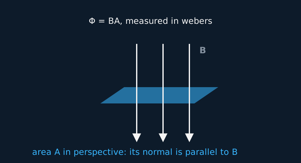
Theory: Magnetic flux and flux linkage
What you are trying to do
Use a search coil and an oscilloscope to show that the flux linkage through a coil follows the cosine of the angle between the coil's normal and the field.
Apparatus
- A large field coil driven by an ac signal generator, producing an alternating field of fixed amplitude at its centre
- A small search coil of many turns on an insulating handle, mounted on a protractor so its angle can be set
- An oscilloscope to read the amplitude of the induced emf
Variables
- Independent: the angle θ between the search coil's normal and the field
- Dependent: the amplitude of the induced emf on the oscilloscope
- Control: the field amplitude and frequency, and the search coil's position at the centre of the field coil
Method
- Drive the field coil with a steady ac signal; the alternating field induces an emf in the search coil whose amplitude is proportional to its flux linkage.
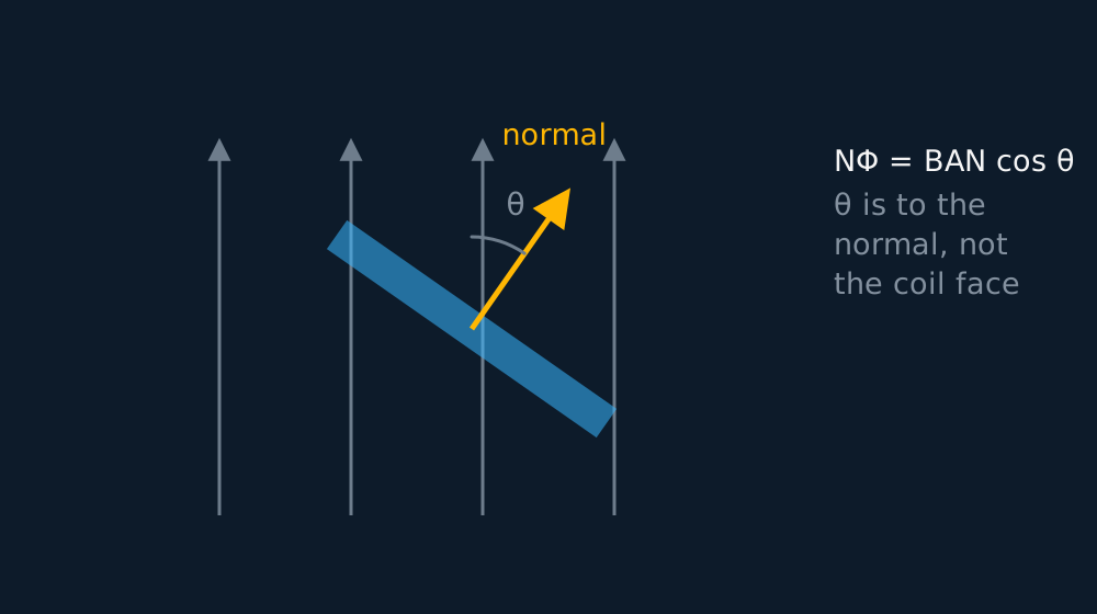
- Centre the search coil where the field is uniform, set θ = 0 (coil face-on), and record the peak-to-peak height of the trace.
- Rotate in steps of fifteen degrees to ninety, recording the amplitude at each angle without moving the coil's centre.
Analysis
- The linkage is NΦ = BANcos θ, and the induced amplitude is proportional to it, so plot the amplitude against cos θ.
- Fit the line without constraining the intercept. A straight line through the origin supports the model: linkage, and with it the induced emf, follows the cosine of the angle to the normal. Report any residual amplitude at 90° rather than forcing a zero intercept, which is justified only if the residual is small compared with the scatter of the readings.
- What the line gives you, and what it does not. Straight and through the origin, it supports NΦ = BANcos θ over the quarter turn you covered. It does not give B, because the gradient carries N and A along with it, and it says nothing about frequency, which you held fixed. If you want the cosine tested over more of its shape, keep turning past ninety degrees towards a hundred and eighty and watch the amplitude grow again as the linkage rebuilds with the opposite sign. An amplitude reading alone cannot show that reversal; seeing the sign change needs a phase reference, such as the drive signal on the scope's second channel.
- Where this method is weakest. Near 90°, the predicted signal changes rapidly with angle but its absolute amplitude is small, so background pickup and oscilloscope resolution produce a large fractional uncertainty. No amount of care with the protractor changes that. Recording the trace with the field coil switched off measures the pickup instead of hiding it. Subtracting amplitudes is valid only if the pickup is in phase with the wanted signal: two signals differing in phase do not subtract arithmetically, so put the drive signal on the oscilloscope's second channel as a phase reference before correcting anything.
A worked set of readings
Amplitudes from the oscilloscope at fifteen-degree steps:
| θ / ° | cos θ | Amplitude / V |
|---|---|---|
| 0 | 1.000 | 4.00 |
| 15 | 0.966 | 3.86 |
| 30 | 0.866 | 3.46 |
| 45 | 0.707 | 2.83 |
| 60 | 0.500 | 2.00 |
| 75 | 0.259 | 1.04 |
| 90 | 0.000 | 0.00 |
Idealised illustrative data, chosen so the working is easy to follow. Real readings scatter about the line rather than sitting on it, and your own graph will have points either side of the best fit.
Amplitude against cos θ is a straight line through the origin with gradient 4.00 V, the face-on amplitude: linkage follows BANcos θ exactly as the model says.
Evaluating the result
Idealised readings, except the last, which is what a real search coil shows. Edge on, the flux linkage is zero and the model predicts no signal at all, but the trace does not collapse to a flat line: mains fields and the leads themselves induce something. Every other row here is 4.00 V times cos θ.
| θ / ° | cos θ | Amplitude / V |
|---|---|---|
| 0 | 1.000 | 4.00 |
| 45 | 0.707 | 2.83 |
| 75 | 0.259 | 1.04 |
| 90 | 0.000 | 0.20 |
Idealised illustrative data, chosen so the working is easy to follow. Real readings scatter about the line rather than sitting on it, and your own graph will have points either side of the best fit.
The first three rows sit on the cosine and the last reads 0.20 V where the model says zero. Retain that reading and report it rather than deleting it. Switch the field coil off and look again: if 0.20 V is still there, it is background pickup and belongs in the evaluation; if it disappears, the coil was not truly edge-on. Compare the phase of the residual with the drive signal before subtracting it, because amplitudes that differ in phase do not subtract arithmetically. On the amplitude against cos θ graph the residual lifts the line off the origin, and a line forced through zero would hide that offset instead of reporting it.
Where the uncertainty comes from
- Angle setting: A protractor mount reads to a degree or two; the cosine is flattest near zero, so errors there matter least, and most near ninety degrees.
- Position drift: The field is uniform only near the centre of the field coil; rotating without translating is the manual skill.
- Reading the trace: Use peak-to-peak and halve it: the full height is easier to judge against the graticule than a single peak.
- Amplifier and coupling: Keep the oscilloscope settings fixed from first reading to last so every amplitude is on the same scale.
What earns the marks
✓Marks
- Define θ from the field to the coil's normal, and say that face-on gives maximum linkage. Measuring the angle to the coil's face instead reverses the trend.
- Plot against cos θ to linearise, and state whether the fitted line passes through the origin within the scatter of the readings.
- Peak-to-peak halved, with the scope's volts-per-division stated.
- Know why an ac field is needed at all: a steady flux linkage induces nothing; it is the changing flux that drives the emf.
Safety
!Caution
Signal-level voltages throughout, so the electrical risk is low. The field coil can warm with sustained drive, so switch off between runs.
Method and analysis here follow the standard approach; your school may vary the apparatus. Always follow your teacher’s risk assessment in the lab.