Physics › Required practicals › Simple harmonic motion: mass-spring and pendulum
REQUIRED PRACTICAL 7Simple harmonic motion: mass-spring and pendulum
Timing a simple pendulum and a mass on a spring, and finding g and k from graphs of T² against length and against mass.
Theory: The mass on a spring and the simple pendulum
What you are trying to do
Investigate simple harmonic motion with the two standard oscillators: a simple pendulum, and a mass on a spring.
Apparatus
- String and a small dense bob; a clamp stand tall enough for lengths up to a metre or more
- A spring, slotted masses and hanger
- Stopwatch, metre rule, and a fiducial marker (a pin or card at the equilibrium position)
Variables
- Independent: the pendulum's length l; the oscillating mass m on the spring
- Dependent: the period T
- Control: small amplitudes throughout; the same spring; the same bob
Method

- Place the fiducial marker at the equilibrium position, start the oscillation with a small displacement, and time twenty complete cycles from a centre crossing. Divide by twenty, and repeat each timing.
- For the pendulum, vary l over at least five values, measuring to the centre of the bob. Keep the swing under about ten degrees.
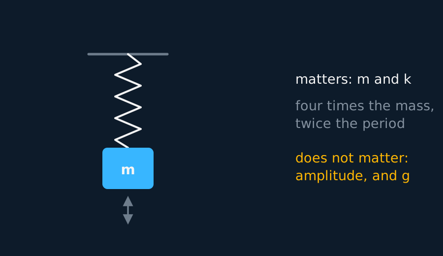
- For the spring, vary the load over five values, displacing vertically by a small amount each time.
Analysis
- Plot T² against l for the pendulum and T² against the total oscillating mass m, hanger included, for the spring. Fit an unconstrained straight line to each. The gradients are 4π²/g and 4π²/k; a significant intercept may indicate a length zero error or the spring's effective mass.
- Squaring the period linearises T = 2π√(l/g) and T = 2π√(m/k), so the gradient of each line is set by all the readings rather than by one pair.
- What the pendulum supports, and what the spring adds. A value of g within a per cent or two of 9.81 m s⁻² supports T = 2π√(l/g) over the lengths you tried, which is a stronger statement than any single timing could make. The spring gives k, and that one can be measured a second way: hang a load on the same spring, measure the extension it settles at, and compare k from F = kx with k from the timings. Agreement between the static and dynamic values supports the consistency of the two measurements; it does not prove the model, since both rest on the same assumption that the spring obeys Hooke's law over this range.
- The model's own limit. Isochrony is a small-angle result, so this procedure cannot test the pendulum at large amplitude without breaking the theory it is checking. By twenty degrees the period has crept up by about three quarters of a per cent, and by forty degrees by around three. The spring has its own version: part of the spring oscillates with the load, and its mass shows up as a positive intercept on the T² against m graph. Neither is a mistake to be tidied away: report the intercept rather than forcing the line through the origin.
A worked set of readings: the pendulum
Each T is the mean of two timings of twenty oscillations:
| l / m | T / s | T² / s² |
|---|---|---|
| 0.400 | 1.269 | 1.610 |
| 0.600 | 1.554 | 2.415 |
| 0.800 | 1.794 | 3.219 |
| 1.000 | 2.006 | 4.024 |
| 1.200 | 2.198 | 4.829 |
Idealised illustrative data, chosen so the working is easy to follow. Real readings scatter about the line rather than sitting on it, and your own graph will have points either side of the best fit.
The gradient of T² against l is 4.024 s² m⁻¹, and g = 4π²/gradient = 9.81 m s⁻².
A worked set of readings: the spring
Same timing routine, five loads:
| m / kg | T / s | T² / s² |
|---|---|---|
| 0.100 | 0.397 | 0.158 |
| 0.200 | 0.562 | 0.316 |
| 0.300 | 0.688 | 0.474 |
| 0.400 | 0.795 | 0.632 |
| 0.500 | 0.889 | 0.790 |
Idealised illustrative data, chosen so the working is easy to follow. Real readings scatter about the line rather than sitting on it, and your own graph will have points either side of the best fit.
The gradient of T² against m is 1.579 s² kg⁻¹, so k = 4π²/gradient = 25.0 N m⁻¹.
Evaluating the result
Idealised pendulum readings with one timing miscounted. At 0.800 m the count started at one instead of zero, so nineteen swings were timed and the total was still divided by twenty. The third column divides T² by l, which the model says is 4π²/g at every length.
| l / m | T / s | T²/l / s² m⁻¹ |
|---|---|---|
| 0.400 | 1.269 | 4.02 |
| 0.600 | 1.554 | 4.02 |
| 0.800 | 1.705 | 3.63 |
| 1.000 | 2.006 | 4.02 |
Idealised illustrative data, chosen so the working is easy to follow. Real readings scatter about the line rather than sitting on it, and your own graph will have points either side of the best fit.
Three rows give 4.02 s² m⁻¹ and the miscounted one gives 3.63, low by 9.8 per cent, because a five per cent error in T becomes ten per cent in T². On the T² against l graph the point sits below the line. The size of the drop is what separates the explanations: one swing missed in twenty lowers the plotted value by about a tenth at every length, while a misjudged crossing or a mismeasured length moves one point by much less. Time that length again, starting the count at zero as the bob passes the marker, and keep both timings in the table with the reason the first was excluded.
Where the uncertainty comes from
- Timing: Human reaction is about 0.2 s; spreading it over twenty cycles cuts it twentyfold, and the fiducial marker at the centre sharpens the start and stop.
- Length: To the centre of the bob, not the top: half a bob diameter is a systematic error otherwise.
- Amplitude: The pendulum's isochrony is a small-angle result; beyond about ten degrees the period creeps up.
- The spring's own mass: A real spring carries some of its own mass along; it shows up as a small positive intercept on the T² against m graph, another reason not to force the line through the origin.
What earns the marks
✓Marks
- Twenty oscillations, timed from the equilibrium position past a fiducial marker, repeated and averaged: state all three parts.
- Plot T², not T, and state what each gradient is: 4π²/g for the pendulum and 4π²/k for the spring.
- Measure the pendulum to the bob's centre and keep the amplitude small, and say why for both.
- Interpret intercepts physically (spring mass, length offset) rather than forcing lines through the origin.
Safety
!Caution
A loaded spring can fly if it slips its support, and slotted masses land hard: clamp the stand, keep the stack modest, and keep eyes out of the line of a stretched spring.
Method and analysis here follow the standard approach; your school may vary the apparatus. Always follow your teacher’s risk assessment in the lab.