Maths › Algebra and functions › Graphs, proportion and transformations
Graphs, proportion and transformations
Sketch polynomial, reciprocal and rational functions from their roots, repeated factors, discontinuities, asymptotes and end behaviour. Apply translations, stretches and reflections, sketch 1/f(x), and use a discriminant to determine the range of suitable rational functions.
Builds on Polynomials and the factor theorem.
IN THIS TOPIC
- Sketch a cubic or quartic from its factors, with crossings and touches in the right places.
- Sketch y = a/x and y = a/x2 and state their asymptotes.
- Set up direct, inverse and inverse-square proportion, and fit the constant from one data point.
- Apply the four transformations of y = f(x), singly and in combination.
- Sketch y = 1/f(x) from a given curve, trading zeros for asymptotes and turning points for their reciprocals.
- Diagnose a rational curve from its coefficients, oblique asymptotes included, and find where it meets a straight line.
- Find the range and the stationary points of a rational function from a discriminant rather than a derivative.
- Count the solutions of f(x) = k from where the line y = k crosses the curve.
COMMON MISCONCEPTION
Replacing x by (x + a) moves the graph a units to the right.
y = f(x + a) translates the graph a units to the left. Adding inside the bracket feeds the function an x from further to the right, so the picture slides the other way. Changes outside the bracket act on y and do what they say; changes inside act on x and do the opposite, which is why y = f(ax), for a > 0, is a horizontal stretch of scale factor 1/a.
Sketching from the factors
A polynomial in factorised form can be sketched directly. The leading term fixes the end behaviour, so a positive cubic runs from bottom-left to top-right and a positive quartic from top-left to top-right, and each factor gives a root. The power of the factor determines the behaviour at that root: a simple factor crosses the axis, and a squared factor touches it, as (x + 2)2 does in the cubic x3 + 3x2 − 4.
WORKED EXAMPLE
A cubic read straight off its factors
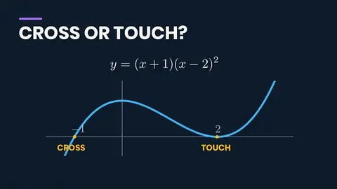
Sketch y = (x + 1)(x − 2)2, marking every axis meeting.
Roots first. A crossing at x = −1 from the simple factor, a touch at x = 2 from the squared one.
The y-intercept comes from x = 0, namely 1 × 4 = 4.
A positive cubic with those features increases through x = −1, turns, meets the axis at x = 2 without crossing it, and then increases. No table of values is required.
An intersection of two curves is a solution of the corresponding pair of equations, so the number of crossings on a sketch is the number of solutions.
Reciprocal curves and proportion
The graphs of y = a/x and y = a/x2 introduce the asymptote, a line the curve approaches: the distance between curve and line tends to zero. Both axes are asymptotes here. As x tends to 0 the functions are unbounded, and as |x| increases the curves approach the horizontal axis.
An asymptote is defined by that limiting behaviour, not by the curve never meeting the line. A curve may cross its own asymptote: y = (sin x)/x crosses y = 0 infinitely often and still approaches it, because the amplitude of the oscillation tends to zero. These two reciprocal curves do not meet their axes, but that is a property of these curves rather than part of the definition.
Sign is what separates the two, and a carries a sign of its own. For y = a/x the sign of y is the sign of a times the sign of x, so a positive a puts the branches in the first and third quadrants and a negative a puts them in the second and fourth. Either way there is one branch in each of two opposite quadrants. For y = a/x2 the square makes the denominator positive, so y takes the sign of a alone. Both branches then sit on one side of the horizontal axis, above it when a is positive and below it when a is negative.
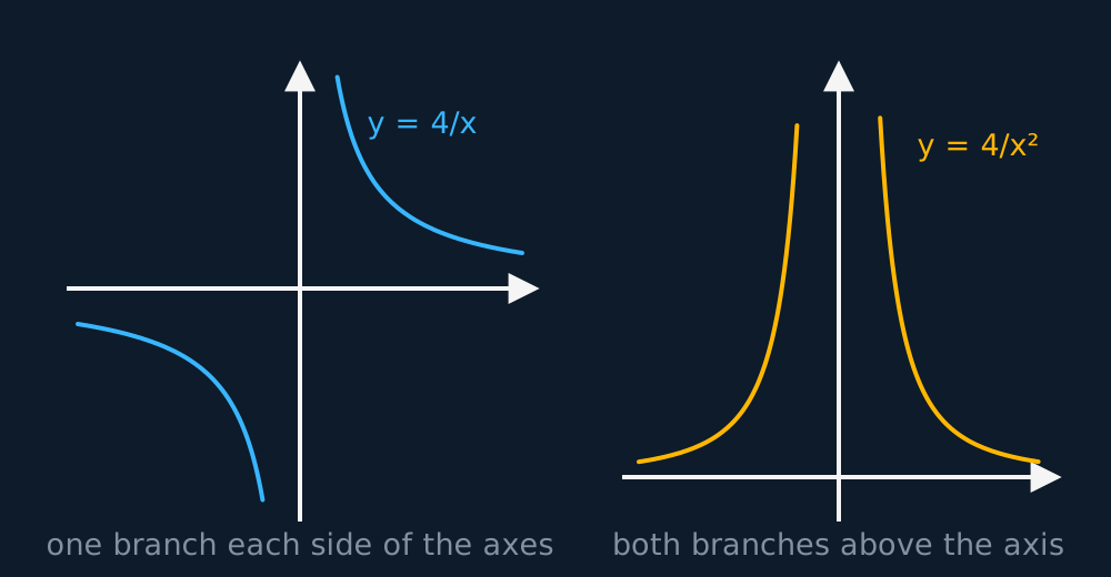
These are also the curves of proportion. Direct proportion, y = kx, is a straight line through the origin. Inverse proportion, y = k/x, is the reciprocal curve. Inverse square, y = k/x2, is its one-sided cousin. One data point fixes k and the whole curve follows.
WORKED EXAMPLE
Inverse square proportion, pinned by one point
y is inversely proportional to x2, and y = 4 when x = 3. Find y when x = 2.
Write the relationship with a constant, y = k/x2, then substitute the known pair. k = 4 × 9 = 36.
So y = 36/x2, and at x = 2, y = 36/4 = 9.
y varies as the inverse square of x, so halving x multiplies y by 4.
The four transformations
Four transformations of y = f(x) are required by Edexcel 9MA0 2.9. The two stretches are stated below for a > 0; the case a < 0 is treated in the paragraph that follows.
| Equation | Effect on the graph of y = f(x), for a > 0 |
|---|---|
| y = f(x) + a | translate a units up |
| y = f(x + a) | translate a units to the left |
| y = af(x) | stretch ×a vertically |
| y = f(ax) | stretch ×1/a horizontally |
A negative a needs one extra word. y = af(x) is a stretch of scale factor |a| vertically and a reflection in the x-axis, and y = f(ax) is a stretch of scale factor 1/|a| horizontally and a reflection in the y-axis. So y = −2f(x) doubles every height and then flips the picture upside down. Do not describe it as a stretch of scale factor −2. The translations need no such caution, since a negative a there simply translates the other way. Zero is the dead end. y = 0f(x) flattens the whole curve onto the x-axis, and y = f(0x) is the constant f(0), so neither is a stretch and neither can be undone.
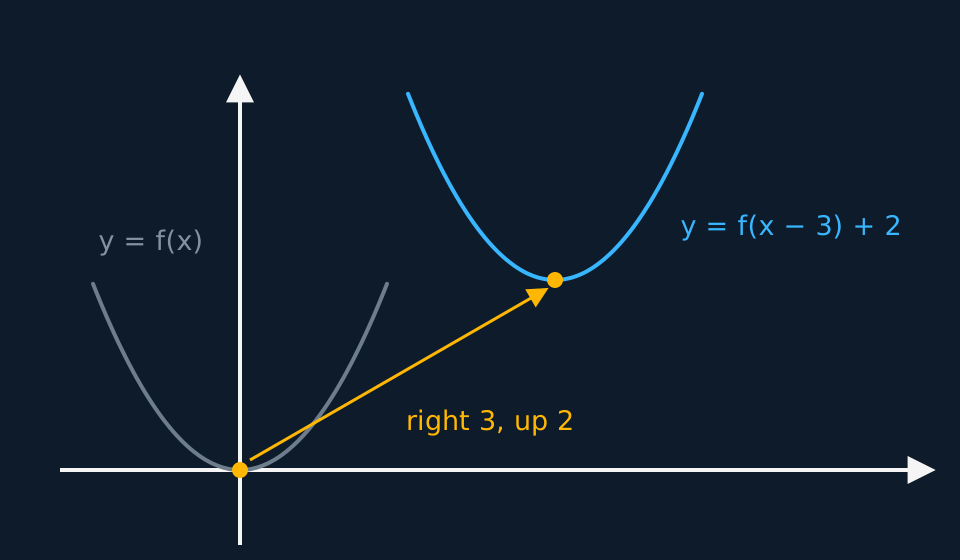
The second row is the counter-intuitive one. Adding inside the bracket feeds the function an x from further to the right, so the picture slides left, not right. Changes outside the bracket act on y and do what they say. Changes inside act on x and do the opposite.
WORKED EXAMPLE
Tracking a single point
The curve y = f(x) passes through (2, 5). Find the corresponding point on y = f(x − 1) + 3.
Inside the bracket, x − 1 must equal 2, so x = 3. The picture has moved right by 1.
Outside, 3 is added to the output, lifting 5 to 8. The point is (3, 8).
Tracking one point through the substitution determines the transformation without relying on memorised rules.
Combinations, and the order they happen in
Where a stretch and a translation act in the same direction, the order in which they are applied matters: af(x) + b and a(f(x) + b) are different curves, and the same holds inside the bracket, where f(2x + 6) is the standard case.
GUIDED PRACTICE
A transformed reciprocal
Sketch y = 1/(x − 2) + 1, stating the equations of its asymptotes and where it meets the axes, before opening the working.
Show the working
Start from y = 1/x and read the moves. Right 2, up 1, so the asymptotes travel too, to x = 2 and y = 1.
Axis meetings come from the equation. At x = 0, y = −1/2 + 1 = 1/2. Setting y = 0 gives 1/(x − 2) = −1, so x = 1.
The curve meets the axes at (0, 1/2) and (1, 0), with one branch below-left of the asymptote crossing and one above-right.
Draw the transformed asymptotes as dashed lines first, then place each branch relative to them using the signs and a few points.
INDEPENDENT PRACTICE
A combination, in the right order
The curve y = f(x) has a root at x = 0. Describe two correct sequences of transformations taking y = f(x) to y = f(2x + 6), and state where the root ends up.
Show the working
Read f(2x + 6) as f(2(x + 3)). One route translates 6 left, then stretches horizontally ×1/2. The other stretches ×1/2 first, then translates only 3 left.
Either way the root lands where 2x + 6 = 0, at x = −3.
Stretching first and then translating 6 units left puts the root at x = −6, which does not satisfy 2x + 6 = 0, so that sequence is incorrect.
The reciprocal of a curve
A curve can also be sketched from another curve. For the reciprocal y = 1/f(x), each feature follows from one fact: taking the reciprocal of a non-zero value inverts its size and preserves its sign, so small values become large and large values become small.
| On the curve y = f(x) | On the curve y = 1/f(x) |
|---|---|
| a crossing of the x-axis | a vertical asymptote |
| a vertical asymptote | a crossing of the x-axis |
| the height grows without bound | the curve flattens onto y = 0 |
| a maximum, on a stretch of one sign | a minimum there, at the reciprocal height |
| the height is 1 or −1 | the two curves meet |
The sign determines which side of the horizontal axis each part of the new curve lies on. Where f is positive so is 1/f, and where f is negative so is 1/f, so the reciprocal keeps to the side of the axis the original was on. That is also why the turning points swap type instead of moving: along a stretch where f holds one sign, a maximum of f is a minimum of 1/f at the reciprocal height, and a minimum of f is a maximum of 1/f.
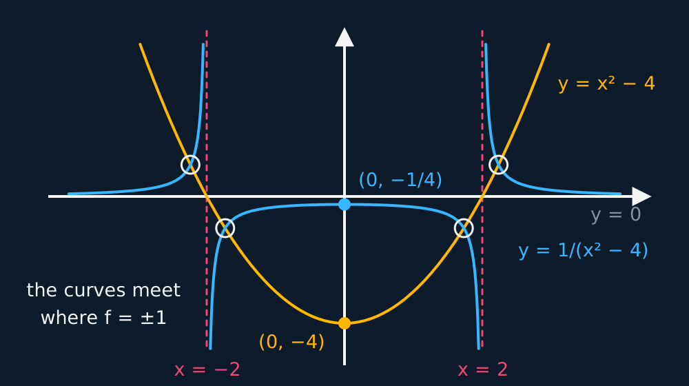
The figure below shows a parabola and its reciprocal on the same axes.
Describe the drawing
The parabola y = x² − 4 and its reciprocal on one pair of axes. Each zero of the parabola, at minus 2 and 2, has become a dashed vertical asymptote of the reciprocal; the parabola's minimum at (0, −4) has become a maximum at (0, −1/4) on the same side of the axis; the far arms of the parabola climb away while the outer branches of the reciprocal flatten onto y = 0; and the four ringed points are where the parabola stands at 1 or −1, the only heights at which a curve and its reciprocal can meet.
WORKED EXAMPLE
A parabola, turned upside down
The curve y = x2 − 4 is given. Sketch y = 1/(x2 − 4), marking its asymptotes and its turning point.
Zeros first. The parabola crosses at x = −2 and x = 2, so the reciprocal has vertical asymptotes x = −2 and x = 2.
As |x| increases the parabola is unbounded, so its reciprocal tends to zero and the curve approaches y = 0.
The parabola's minimum is (0, −4), and the sign is kept, so the reciprocal has a maximum at (0, −1/4).
The two curves meet where x2 − 4 is 1 or −1, that is at x = ±√5 and x = ±√3, which pins the middle of the sketch.
Between −2 and 2 the parabola is negative, so this part of the reciprocal lies below the axis, with a maximum at −1/4 and unbounded negative values near both asymptotes. Outside that interval the two parts are positive and tend to zero.
Rational curves, read off the coefficients
A rational function is one polynomial over another. Use numerator roots for zeros, uncancelled denominator roots for vertical asymptotes, cancelled factors for holes, and polynomial division or leading terms for end behaviour. These determine the main features; use further points, inequalities or derivatives where needed.
| Feature | Where it comes from |
|---|---|
| the zeros | roots of the numerator that are not also roots of the denominator |
| the vertical asymptotes | roots of the denominator that do not cancel |
| the holes | factors common to numerator and denominator, which cancel |
| the end behaviour | the two degrees: equal degrees give the ratio of the leading coefficients, a lower-degree numerator gives y = 0, and a numerator one degree higher gives an oblique asymptote |
Cancel any common factor before reading the features. At a cancelled value of x the curve has a hole rather than a vertical asymptote.
Take the linear-over-linear case y = (ax + b)/(cx + d), with c non-zero. The denominator is zero at x = −d/c, which gives the vertical asymptote. As |x| increases the constants b and d become negligible beside the terms in x, so y tends to a/c and the horizontal asymptote is y = a/c. Dividing out gives both at once: the quotient is the constant a/c and the remainder term is a multiple of 1/(cx + d), so the curve is y = 1/x stretched and translated.
WORKED EXAMPLE
A rational curve, a line, and the inequality between them
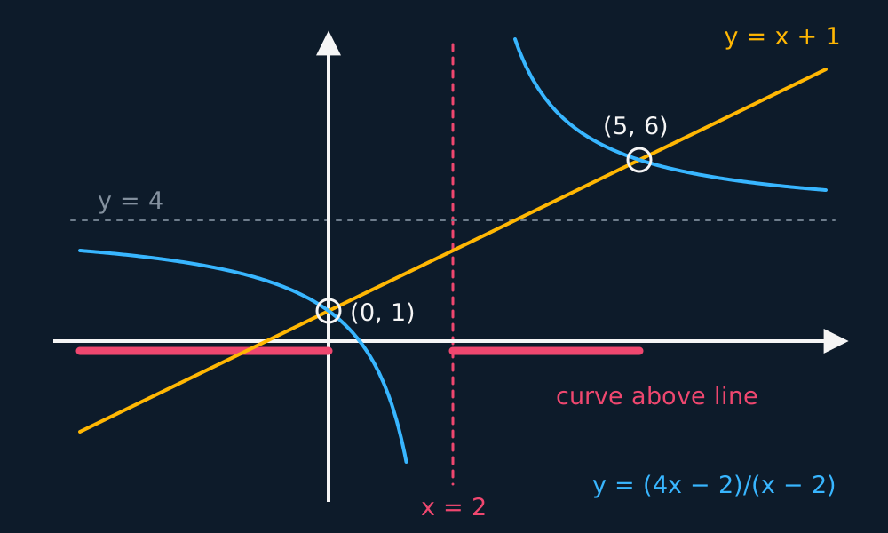
Sketch y = (4x − 2)/(x − 2), giving its asymptotes and axis crossings. Find where it meets y = x + 1, and hence solve (4x − 2)/(x − 2) > x + 1.
The bottom vanishes at x = 2, and the leading coefficients are 4 and 1, so the asymptotes are x = 2 and y = 4.
Crossings. Setting y = 0 needs 4x − 2 = 0, giving (1/2, 0), and x = 0 gives (0, 1).
Dividing out, (4x − 2)/(x − 2) = 4 + 6/(x − 2), so the sketch is y = 6/x moved 2 right and 4 up, with the asymptotes carried along.
Meeting the line. Multiply up: 4x − 2 = (x + 1)(x − 2) = x2 − x − 2, so x2 − 5x = 0 and x = 0 or x = 5. The two points are (0, 1) and (5, 6).
For the inequality, subtract and combine rather than multiplying by x − 2, whose sign is unknown: (4x − 2)/(x − 2) − (x + 1) = x(5 − x)/(x − 2). The critical values are 0, 2 and 5, and testing the four intervals gives x < 0 or 2 < x < 5.
The sketch gives the same solution set: the curve lies above the line to the left of the origin, and again on the branch between the vertical asymptote and the second crossing.
The curve, the line and the two intervals named by the inequality are drawn together below.
Describe the drawing
The curve y = (4x − 2)/(x − 2) with the line y = x + 1 laid across it. The dashed vertical x = 2 splits the curve into two branches and the dashed horizontal y = 4 is the height it settles onto; the line cuts the left branch at (0, 1) and the right branch at (5, 6), both ringed. The two coral bars on the axis mark the stretches x < 0 and 2 < x < 5, which are exactly the x for which the curve is drawn above the line, so the sketch solves the inequality by inspection.
GUIDED PRACTICE
The general case, sketched
Sketch y = (3x + 6)/(x − 1), stating its asymptotes, its axis crossings and the translated reciprocal curve it turns out to be, before opening the working.
Show the working
The bottom vanishes at x = 1, and the leading coefficients are 3 and 1, so the asymptotes are x = 1 and y = 3.
Setting y = 0 gives x = −2, and x = 0 gives y = −6, so it crosses at (−2, 0) and (0, −6).
Dividing out, 3(x − 1) + 9 = 3x + 6, so y = 3 + 9/(x − 1), which is y = 9/x translated 1 right and 3 up.
The two methods give the same asymptotes. State them as equations, x = 1 and y = 3, rather than as bare numbers.
The same readings apply at higher degree. The curve y = (ax2 + bx + c)/(dx2 + ex + f) has a vertical asymptote at each root of the denominator, so up to two, a zero at each root of the numerator, and it tends to y = a/d, the ratio of the leading coefficients. A curve of this form may meet its horizontal asymptote; subtracting that value from the function shows whether it does.
WORKED EXAMPLE
Two quadratics
Sketch y = (x2 − 4)/(x2 − 1), stating its asymptotes and where it crosses the axes.
The bottom vanishes at x = ±1, so the vertical asymptotes are x = 1 and x = −1. The top vanishes at x = ±2, so the curve crosses at (−2, 0) and (2, 0), and x = 0 gives (0, 4).
The leading coefficients are 1 and 1, so the horizontal asymptote is y = 1.
To test whether the curve attains that value, subtract it: y − 1 = (x2 − 4 − x2 + 1)/(x2 − 1) = −3/(x2 − 1). A fraction with a non-zero constant numerator is never zero, so the curve approaches y = 1 without meeting it.
The same expression gives which side of the asymptote each part lies on. Outside the vertical asymptotes x2 − 1 is positive, so y − 1 is negative and the two outer parts lie below y = 1; between them x2 − 1 is negative, so the middle part lies above y = 1 and passes through (0, 4).
Any of those six coefficients may be zero, and two cases change the end behaviour. A numerator of lower degree than the denominator gives the horizontal asymptote y = 0. A denominator of lower degree gives the remaining case, treated next.
When the top's degree is the larger, divide. A quadratic over a linear bracket leaves a linear quotient and a proper remainder term, and that term tends to zero as |x| increases, so the curve approaches the line the quotient names. That line is the oblique asymptote. A similar idea gives the slanting asymptotes of a hyperbola: keeping the dominant terms and dropping the constant leaves the pair of lines the branches approach. The algebraic division of an improper fraction from Polynomials and the factor theorem is what produces the quotient here.
WORKED EXAMPLE
An asymptote that slants
Sketch y = (x2 + x − 2)/(x − 2), giving its asymptotes and its axis crossings.
The top factorises as (x + 2)(x − 1), so the curve crosses at (−2, 0) and (1, 0), and x = 0 gives (0, 1). The bottom vanishes at x = 2, so x = 2 is a vertical asymptote.
The top outranks the bottom by one degree, so divide: x2 + x − 2 = (x − 2)(x + 3) + 4, which gives y = x + 3 + 4/(x − 2).
The remainder term tends to zero as |x| increases, so the curve approaches y = x + 3, the oblique asymptote.
The remainder term also gives which side of the line the curve lies on. For x > 2 it is positive and the curve lies above the line; for x < 2 it is negative and the curve lies below. At x = 50 the difference is 4/48, about 0.08, and it decreases as x increases.
Which heights a rational curve reaches
The set of values the function takes can be found without calculus, by quadratic theory. A value k is in the range exactly when the line y = k meets the curve, so set the expression equal to k, clear the fraction, and require the resulting quadratic in x to have a real root. The condition that its discriminant is non-negative gives an inequality in k, which is the range.
The stationary points follow from the same working. At each end of the range the discriminant is zero, so the quadratic has a repeated root and the horizontal line y = k is a tangent to the curve. Substituting that value of k back into the quadratic gives the repeated root, which is the x-coordinate of the stationary point.
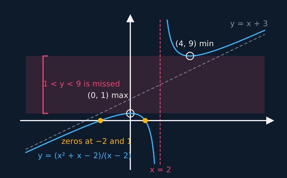
The curve y = (x2 + x − 2)/(x − 2) is drawn below, showing the interval of heights it does not reach. The worked example that follows obtains that interval from the discriminant.
Describe the drawing
The curve y = (x² + x − 2)/(x − 2), drawn with the dashed vertical x = 2 it blows up at and the dashed slanting line y = x + 3 its two branches settle onto far from the origin. The zeros at −2 and 1 are marked, the stationary points (0, 1) and (4, 9) are ringed, and the shaded strip between those two heights is bracketed: the left branch never rises above 1 and the right branch never falls below 9, so the band between them is exactly the set of heights the discriminant argument rules out.
WORKED EXAMPLE
A range and two stationary points, without differentiating
For y = (x2 + x − 2)/(x − 2), find the set of values y can take and the coordinates of the stationary points.
Put the expression equal to k and clear the fraction: x2 + x − 2 = k(x − 2), so x2 + (1 − k)x + (2k − 2) = 0.
A real x needs a non-negative discriminant: (1 − k)2 − 4(2k − 2) = k2 − 10k + 9 = (k − 1)(k − 9) ≥ 0.
That is an upward parabola in k, non-negative outside its roots, so y ≤ 1 or y ≥ 9. No value strictly between 1 and 9 is attained, which is the gap between the two branches either side of x = 2.
The ends give the stationary points. At k = 1 the quadratic is x2 = 0, so x = 0 and the point is (0, 1). At k = 9 it is x2 − 8x + 16 = 0, so x = 4 and the point is (4, 9).
The first is a maximum on the left branch and the second a minimum on the right. The maximum is lower than the minimum because the vertical asymptote separates the two branches, and neither point required differentiation.
INDEPENDENT PRACTICE
A quadratic over a quadratic
Find the set of values y = (2x2 + 4x − 1)/(x2 + 1) can take, and the coordinates of its stationary points.
Show the working
Putting the expression equal to k and clearing gives (2 − k)x2 + 4x − (1 + k) = 0.
Treat k = 2 on its own, since the squared term goes with it. What is left is 4x − 3 = 0, so x = 3/4 and the height 2 is reached.
Otherwise the discriminant is 16 + 4(2 − k)(1 + k) = −4(k − 3)(k + 2), and asking for it to be non-negative gives (k − 3)(k + 2) ≤ 0, that is −2 ≤ y ≤ 3.
At k = 3 the quadratic is −x2 + 4x − 4 = 0, so x = 2 and the maximum is (2, 3). At k = −2 it is 4x2 + 4x + 1 = 0, so x = −1/2 and the minimum is (−1/2, −2).
The horizontal asymptote is y = 2, the ratio of the leading coefficients, and it lies inside the range. The case k = 2 above is the curve meeting that asymptote, at x = 3/4, which is an instance of the definition given earlier: an asymptote is a line the curve approaches, not one it cannot meet.
ASSESSMENT FOCUS
- Sketch from factors in three steps: end behaviour from the leading term, roots from the brackets, y-intercept from x = 0. Label all three on the sketch.
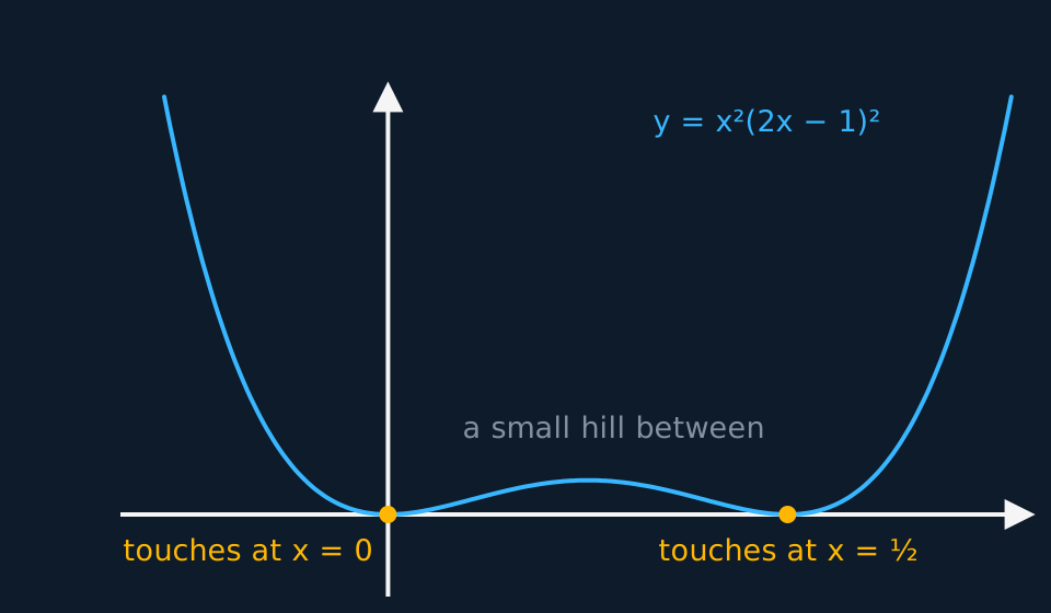
- A squared factor gives a point where the curve touches the axis; a simple factor gives a crossing. A curve such as x2(2x − 1)2 touches the axis at both of its roots.
- Draw asymptotes dashed and state their equations in full, x = 2 and y = 1, never the bare numbers on their own.
- In a proportion question, find the constant first: write y = k/x2, determine k from the given pair of values, then use the fitted equation.
- A change inside the bracket acts horizontally and in the opposite direction; a change outside acts vertically and in the stated direction. For a combination, factorise the inside and track one point through it.
- A pair of sketches answers a “how many solutions” question: each crossing is a solution, and the sketch need only have the correct features.
- For y = 1/f(x), mark the zeros of f as vertical asymptotes, keep the sign of each piece, swap maxima for minima, and add the crossings where f is 1 or −1.
- Diagnose a rational curve before drawing anything: denominator roots for the vertical asymptotes, numerator roots for the zeros, and the two degrees for the end behaviour.
- Divide out whenever the numerator's degree is the larger. The quotient is the oblique asymptote and the sign of the remainder term says which side of it the curve lies.
- Where a range is asked for without calculus, set the expression equal to k, clear the fraction, and require a non-negative discriminant. The endpoints of the resulting inequality are the stationary values, and the repeated root at each endpoint gives the x-coordinate.
- Solve an inequality between a rational curve and a line by subtracting and combining, not by multiplying up. The bracket you would multiply by changes sign at its own asymptote.
CHECK YOURSELF
The curve y = 3/x is transformed to y = 3/x − 2. State the equations of the asymptotes of the new curve, and find where it crosses the x-axis.
Show a hint
The whole curve moves down 2, asymptotes included; then set y = 0.
Show the answer
Subtracting 2 outside translates the curve down 2, so the asymptotes are x = 0 and y = −2.
Setting y = 0 gives 3/x = 2, so x = 3/2, and the curve crosses at (3/2, 0).
The vertical asymptote is unchanged because the transformation acts outside the function. State that reason in the answer.
The factors give the sketch: simple roots cross the axis, repeated roots touch it, and an asymptote is a line the curve approaches, which need not be a line it cannot meet.
Outside the bracket acts on y and does what it says. Inside acts on x and does the opposite.
Under y = 1/f(x) a zero becomes a vertical asymptote and a turning point swaps type at the reciprocal height, with the sign kept.
A rational curve is determined by its zeros, its vertical asymptotes and its end behaviour; divide out when the numerator has the higher degree, and set y = k with a non-negative discriminant to find the range.
WORKBOOK
Printable practice for this topic: original exam-style questions with room to work, and a fully worked answer book. Free to use; please do not redistribute or sell.
Or read them with their worked answers on the graphs, proportion and transformations questions page.
CHECK YOUR PROGRESS
Rate how confident you feel with each objective for this lesson. Ratings are saved in this browser, on this device, unless you sign in.
- Sketch a cubic or quartic from its factors, with crossings and touches in the right places.
- Sketch y = a/x and y = a/x2 and state their asymptotes.
- Set up direct, inverse and inverse-square proportion, and fit the constant from one data point.
- Apply the four transformations of y = f(x), singly and in combination.
- Sketch y = 1/f(x) from a given curve, trading zeros for asymptotes and turning points for their reciprocals.
- Diagnose a rational curve from its coefficients, oblique asymptotes included, and find where it meets a straight line.
- Find the range and the stationary points of a rational function from a discriminant rather than a derivative.
- Count the solutions of f(x) = k from where the line y = k crosses the curve.
Open the full revision checklist to see every objective in the course in one place.