Maths › Statistics › Measures of location and spread
Measures of location and spread
Measures of location summarise the centre of a data set and measures of spread summarise its variability. Calculate the mean, median and quartiles, then the variance and standard deviation, and determine the effect of coding on each.
Builds on Sampling and the large data set.
IN THIS TOPIC
- Find the mean, median and mode of a data set, and say which of them best represents it when one extreme value is present.
- Find the median and quartiles of a listed data set, or of one already ordered by a display, using Edexcel's position rules.
- Estimate the median, quartiles and percentiles of grouped data by linear interpolation.
- Calculate variance and standard deviation from raw data or from the sums Σx and Σx².
- Undo coding to recover the mean and standard deviation of the original variable.
COMMON MISCONCEPTION
Adding 5 to every value in a data set increases the standard deviation.
Adding 5 leaves the standard deviation unchanged. It shifts every value by the same amount, so the mean rises by 5 while the differences between values, and hence σ, stay as they were. Only scaling changes the spread: under the coding y = (x − a)/b, mean(x) = a + b mean(y) and σx = |b|σy.
Location: mean, median, mode
The mean is the total of the values divided by how many there are.
It uses every value, so a single extreme value changes it appreciably. The median is the middle value of the ordered list; it depends only on the order, so extreme values change it little. The mode is the most frequent value, and the only one of the three defined for non-numerical data.
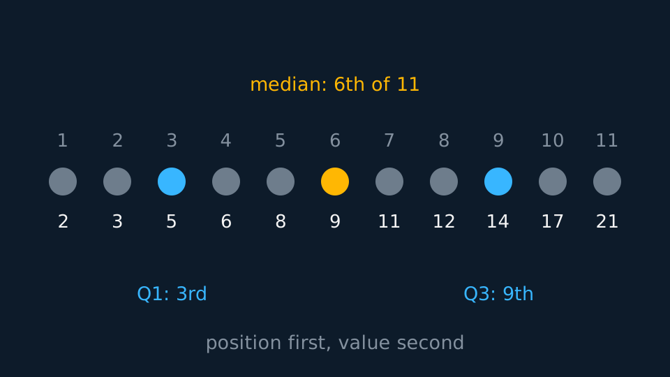
In a list of n values, find positions before you find values. Work out n/4 for Q₁, n/2 for the median and 3n/4 for Q₃. If the position is not a whole number, round it up and read that value. If it is a whole number, take the midpoint of that value and the next one along.
Eleven values put the median at position 5.5, rounded up to the 6th, and Q₁ at 2.75, rounded up to the 3rd. Twelve values put Q₁ at position 3 exactly, so Q₁ is halfway between the 3rd and 4th values. Apply the two cases carefully: they give different values. The interquartile range Q₃ − Q₁ then measures the spread of the middle half.
Where a diagram already presents the data in order, the position rules can be applied to it directly. A stem-and-leaf diagram records the final digit of each value against its leading digits and keeps each row in order, so counting through the rows counts through the ordered data. A dot plot does the same with one dot per observation stacked over an ordered scale.
WORKED EXAMPLE
A median and quartiles from a stem-and-leaf
Fifteen delivery times, in minutes, where 3 | 1 means 31.
| Stem | Leaves |
|---|---|
| 1 | 4 8 |
| 2 | 0 2 2 5 7 |
| 3 | 1 3 4 6 |
| 4 | 0 2 5 |
| 5 | 8 |
Count the rows and keep a running total: 2, 5, 4, 3, 1 leaves, so 2, 7, 11, 14, 15 values so far. Fifteen values puts the median at position 15/2 = 7.5, rounded up to the 8th.
Seven values sit above the 3 row, so the 8th value is that row's first leaf: median = 31 minutes.
Q₁ is at 15/4 = 3.75, rounded up to the 4th value, which is the second leaf of the 2 row, 22. Q₃ is at 45/4 = 11.25, rounded up to the 12th, one past the end of the 3 row and so the first leaf of the 4 row, 40.
IQR = 40 − 22 = 18 minutes. These are exact values rather than estimates, because the diagram retains every individual value.
Grouped data and interpolation
Grouped data does not record the individual values, so the median is estimated under the assumption that the values are distributed uniformly within each class. Accumulate the frequencies up to the class containing position n/2, then add the corresponding fraction of that class width. For grouped data, use n/2 and do not round the position.
WORKED EXAMPLE
A median by interpolation
Masses of 25 parcels, in kg: 8 in the class 10 ≤ m < 20, 12 in 20 ≤ m < 30, and 5 in 30 ≤ m < 40. Estimate the median.
The median position is n/2 = 12.5. The first class carries the count to 8, so the median is the 4.5th of the 12 values inside 20 ≤ m < 30.
Assuming an even spread: median ≈ 20 + (12.5 − 8)/12 × 10 = 20 + 3.75 = 23.75, so about 23.8 kg.
Check: 23.75 lies in the class 20 ≤ m < 30 and less than halfway through it, consistent with 4.5 out of 12.
Quartiles and percentiles are found the same way, with n/4, 3n/4 or, for the 37th percentile, 37n/100 in place of n/2. Identify the class boundaries first: ages given as 20–29 usually mean 20 ≤ a < 30, so the class width is 10 and not 9.
Spread: variance and standard deviation
The range uses two values and ignores the other n − 2. The variance uses all of them: it is the mean of the squared distances from the mean, most usefully calculated in this form.
This is the mean of the squares minus the square of the mean. Check the current formula booklet for your awarding organisation; where the result is supplied it is usually printed as the square root of this expression. The square root of the variance, σ, is the standard deviation, in the units of the data, so quote answers as σ rather than σ². Because the distances are squared, a single distant value increases σ substantially.
WORKED EXAMPLE
Mean and standard deviation from the sums
For 20 values, Σx = 340 and Σx² = 6180. Find the mean and standard deviation.
The mean is 340/20 = 17.
Variance = 6180/20 − 17² = 309 − 289 = 20, so σ = √20 ≈ 4.47.
Check: σ measures a typical distance from the mean, so values four or five units either side of 17 are consistent with these sums.
For grouped data, replace Σx with Σfx and Σx² with Σfx², using class midpoints for x. The result is then an estimate; state that it is an estimate.
Coding
Data are often coded before calculation, by y = (x − a)/b, to make the arithmetic simpler. The summary statistics of x can then be recovered exactly from those of y.
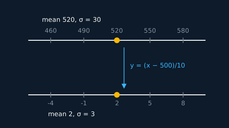
Subtracting a changes every value by the same amount, so the mean changes by a while the differences between values, and hence σ, are unchanged. Dividing by b scales every value, so it divides both the mean and the standard deviation by b.
With y = (x − 500)/10, a coded mean of 3.2 and coded σ of 1.4, the original data have mean 500 + 10 × 3.2 = 532 and σ = 10 × 1.4 = 14. Questions on coding usually ask for the statistics of the original variable, so apply the inverse relations.
ASSESSMENT FOCUS
- A grouped median is an interpolation. Give the class boundaries, the cumulative counts and the fraction of the class width, showing the fraction before evaluating it.
- Use σ² = Σx²/n − (Σx/n)², working directly from the given sums; check the current formula booklet for your awarding organisation, where it is usually printed as a square root under Standard deviation.
- Coding questions usually ask for the original data. Adding a constant changes the mean only; multiplying scales both the mean and σ.
- State which measure suits the context: median and IQR for skewed data or data containing outliers, mean and σ where every value should contribute.
- Quote σ to three significant figures and keep the unrounded value in your calculator for anything that follows.
CHECK YOURSELF
Ten values have Σx = 120 and Σx² = 1560. Find the mean and the standard deviation.
Show a hint
Mean of the squares minus the square of the mean.
Show the answer
Mean: 120/10 = 12.
Variance: 1560/10 − 12² = 156 − 144 = 12, so σ = √12 ≈ 3.46.
Location by position: order the data, find the position, then read the value.
σ² is the mean of the squares minus the square of the mean; scaling the data changes σ, translating it does not.
WORKBOOK
Printable practice for this topic: original exam-style questions with room to work, and a fully worked answer book. Free to use; please do not redistribute or sell.
Or read them with their worked answers on the measures of location and spread questions page.
USED LATER IN
CHECK YOUR PROGRESS
Rate how confident you feel with each objective for this lesson. Ratings are saved in this browser, on this device, unless you sign in.
- Find the mean, median and mode of a data set, and say which of them best represents it when one extreme value is present.
- Find the median and quartiles of a listed data set, or of one already ordered by a display, using Edexcel's position rules.
- Estimate the median, quartiles and percentiles of grouped data by linear interpolation.
- Calculate variance and standard deviation from raw data or from the sums Σx and Σx².
- Undo coding to recover the mean and standard deviation of the original variable.
Open the full revision checklist to see every objective in the course in one place.