Maths › Statistics › Representing and interpreting data
Representing and interpreting data
Choose a diagram according to the data type and comparison required. Use frequency density for histograms, include a key on stem-and-leaf diagrams, apply the outlier rule stated in the question, and interpret skew, quartiles and cumulative-frequency estimates with appropriate precision.
Builds on Measures of location and spread.
IN THIS TOPIC
- Read a stem-and-leaf diagram, a dot plot and a vertical line chart, and say which kind of data each one suits.
- Construct and read histograms using frequency density, including recovering frequencies from areas.
- Draw and compare box plots, and identify outliers using the rule stated in the question.
- Describe skewness from quartiles or from the mean against the median.
- Interpret cumulative frequency diagrams, and clean data before summarising it.
- Choose or criticise a diagram for the job the question is doing.
- Read an unfamiliar diagram through its axes, its key, what one mark represents and a total that can be checked.
COMMON MISCONCEPTION
In a histogram, the height of a bar tells you its frequency.
The height is the frequency density and the area is the frequency. Frequency density is frequency divided by class width, so a bar is read by multiplying its height by its width. A narrow class can stand tallest and hold the fewest values: density 3 across a width of 5 carries 15 observations, against 30 for density 2 across a width of 15.
Diagrams that retain every value
Grouping data discards the individual values. The three diagrams below retain them, and each suits a different kind of data set.
A stem-and-leaf diagram splits every value into a leading part, the stem, and a final digit, the leaf. The stems are listed down the left in order, and each value's leaf is placed against the matching stem, in order along the row. Row lengths then show the shape of the distribution as a bar chart would, and no information is lost: a stem together with any one of its leaves gives back the original value.
| Stem | Leaves |
|---|---|
| 2 | 4 7 9 |
| 3 | 1 3 3 6 8 8 |
| 4 | 0 2 5 5 7 9 |
| 5 | 1 4 6 |
| 6 | 2 |
Nineteen test marks. The key fixes the scale: 4 | 2 means 42. The same rows could otherwise represent 4.2 or 420, so a stem-and-leaf diagram must include a key. The leaves are also written in order, so the diagram presents the data already sorted, which makes it convenient for finding a median.
WORKED EXAMPLE
Reading a stem-and-leaf diagram
For the marks above, find how many candidates sat the test, how many scored 45 or more, and the range.
One leaf is one candidate, so count leaves: 3 + 6 + 6 + 3 + 1 = 19.
Marks of 45 or more are the leaves 5, 5, 7 and 9 on the 4 row, then every leaf on the rows below it: 4 + 3 + 1 = 8 candidates.
The individual values are retained, so the range is exact rather than estimated: 62 − 24 = 38 marks.
Check: the longest rows are in the middle and a single value lies out at 62, so the distribution has a longer tail to the right than to the left.
A dot plot suits a data set small enough to show one observation at a time. Draw the scale, place a dot above the value for every observation, and stack repeated values. Nothing is summarised, so repeats, gaps and an isolated extreme value are all visible. It is printed here one row per value; drawn conventionally the rows become columns above a number line, with the row lengths as the column heights.
| Goals | One dot per match |
|---|---|
| 0 | · · · |
| 1 | · · · · |
| 2 | · · · |
| 3 | · |
| 4 | |
| 5 | · |
Twelve matches. The tallest column is at 1, so the mode is 1. The 6th and 7th values are both 1, so the median is 1. The mean is (4 × 1 + 3 × 2 + 3 + 5)/12 = 18/12 = 1.5, above the median; the plot shows the observation responsible, the single 5 beyond an empty column at 4. A dot plot is suitable at this size and impractical for large data sets.
A vertical line chart applies the same idea to a data set too large to draw dot by dot. The variable is still discrete, so the horizontal axis carries only the values that can occur, but each column of dots becomes a single line whose height is the frequency. The gaps between the lines indicate that no values lie between one possible value and the next, which distinguishes discrete counts from continuous measurements.
| Cars | Height of the line |
|---|---|
| 0 | 5 |
| 1 | 17 |
| 2 | 11 |
| 3 | 5 |
| 4 | 2 |
WORKED EXAMPLE
Reading a vertical line chart
The chart shows the number of cars owned by each of 40 households. Find the mode and the mean number of cars.
Read the heights and add them: 5 + 17 + 11 + 5 + 2 = 40, which matches the 40 households, so no line has been misread.
The tallest line stands at 1, so the mode is 1 car.
The mean is Σfx/Σf = (0 × 5 + 1 × 17 + 2 × 11 + 3 × 5 + 4 × 2)/40 = 62/40 = 1.55 cars.
Check: 1.55 lies between the two most frequent values, 1 and 2, and a mean need not be a whole number of cars.
The choice of diagram follows from the type of data. For categorical data, use a bar chart: the bars are separated because there is nothing between one category and the next, and neither their widths nor their order carries information. For discrete numerical data, use lines at the values that can occur. Continuous data has too many distinct values to show individually, so it is grouped, which leads to the histogram below.
Histograms: area is frequency
A bar chart has equal-width bars, so height alone carries the information. A histogram allows unequal class widths, and each height is then the frequency density.
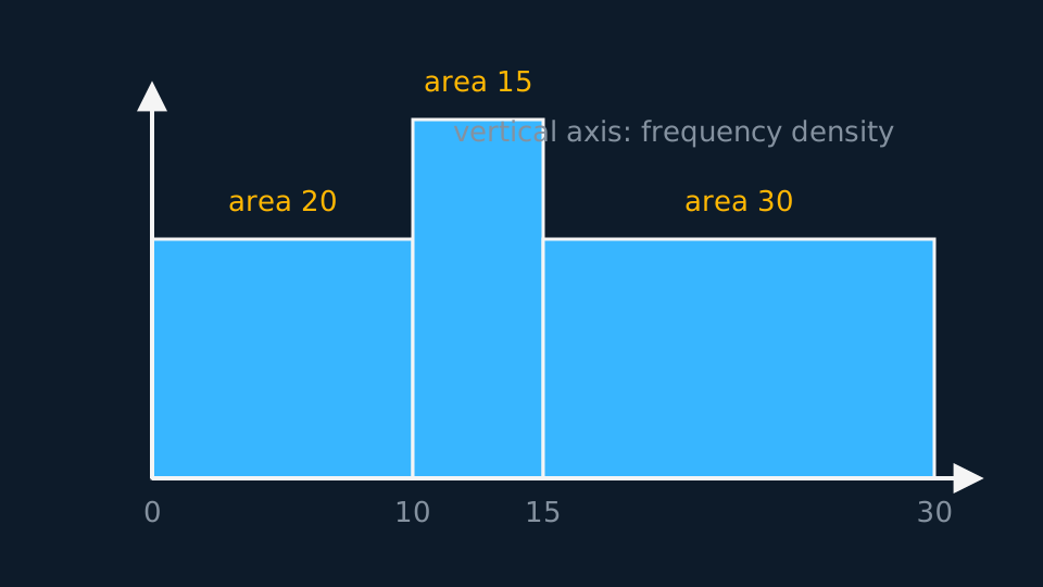
With that vertical scale, area equals frequency. Given a bar, multiply height by width to recover its frequency; given a frequency, divide by the width to obtain the height. A histogram with a key, such as one square representing 5 observations, applies the same relation with a scale factor.
WORKED EXAMPLE
Reading a histogram
In a histogram, the class 15 ≤ x < 30 has frequency 30. The class 10 ≤ x < 15 is drawn with 1.5 times the height of that bar. Find its frequency.
The first bar's density is 30/15 = 2, so the second bar's density is 1.5 × 2 = 3.
Its frequency is density times width: 3 × 5 = 15.
Check by areas. A bar a third as wide but one-and-a-half times as tall carries half the area, 15 against 30, which matches.
A frequency polygon joins the midpoints of the tops of the bars and is commonly used to superimpose two distributions. It shows shape clearly but individual frequencies less precisely, so use it for comparison and a histogram for reading frequencies.
Box plots and outliers
A box plot displays five numbers: the extremes, the quartiles and the median. The box spans the middle half of the data, the median line splits it, and the whiskers reach the most extreme values that are not outliers.
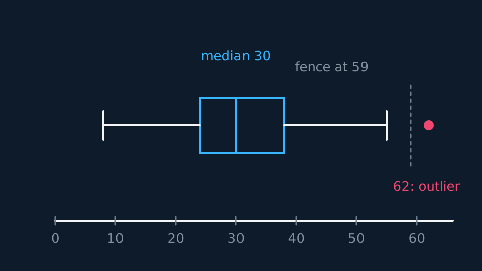
The 1.5 × IQR fences are a common convention, not a definition of an outlier. A question may instead define an outlier as more than two standard deviations from the mean, or supply some other rule. Use the rule stated in the question. An outlier is plotted as a separate cross, and the whisker stops at the most extreme value inside the fence rather than at the fence itself.
Compare two box plots in two sentences: one on location, using the medians, and one on spread, using the IQRs, both expressed in the context of the data. For example: “The median mass is higher for brand A, and brand A's masses are more consistent since its IQR is smaller.”
Shape and skew
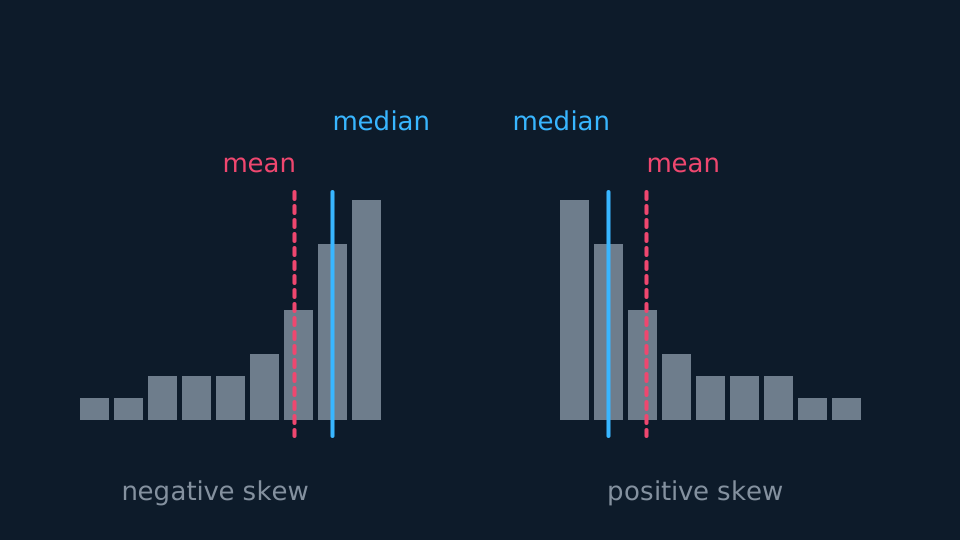
A distribution is symmetric when the median sits midway between the quartiles, so Q₂ − Q₁ = Q₃ − Q₂. When the upper gap is the bigger one, the long tail points right and the data has positive skew. The reverse gives negative skew.
A long right tail and a mean greater than the median are evidence consistent with positive skew. State the feature used; neither comparison is a universal definition of skew. Where the quartile comparison and the mean-median comparison disagree, say so and state which measure of location and spread the data support.
Cumulative frequency
Plot cumulative frequency against the upper class boundary and join the points with a smooth increasing curve. Reading across from n/2, n/4 and 3n/4 gives the median and quartiles. Reading up from two values and subtracting estimates the number of observations in an interval. Every such reading is an estimate, because grouping has removed the exact values; quote it to a precision the graph supports.
Reading an unfamiliar diagram
A question may use a diagram not drawn above: a population pyramid, a cumulative percentage curve, a back-to-back stem-and-leaf diagram, or a histogram whose key states that one square represents five observations. Each can be read by the same procedure.
Read the axes and the key before the shape. The axes state what is plotted against what, and in what units. The key states the scale of the drawing; where a key is given, one mark usually represents more than one observation.
Then establish what a single mark represents: one dot, one leaf, one square, one unit of height or one unit of area. In a histogram a unit of height is a frequency density and only area gives frequency.
Then check a total against a known value. The frequencies should add to the stated n, percentages should total 100, and a cumulative curve should finish level with the total. A failed check indicates that the scale has been misread.
Then answer in the terms of the diagram, and state any assumption needed to read it, such as an assumed class boundary or a uniform distribution within a class.
WORKED EXAMPLE
Reading a back-to-back stem-and-leaf
Twenty runners, nine from team A and eleven from team B, are timed in seconds over the same course. Compare the two medians.
| Team A | Stem | Team B |
|---|---|---|
| 8 5 | 2 | 1 4 6 |
| 7 4 2 0 | 3 | 0 3 8 |
| 6 1 | 4 | 2 5 7 9 |
| 3 | 5 | 4 |
Read the key first. On the right, 2 | 1 means 21 seconds. On the left the leaves are also read outwards from the stem, so the row 8 5 against stem 2 holds 25 and 28, and the smallest value in a left-hand row is the leaf nearest the stem.
One leaf is one runner: 2 + 4 + 2 + 1 = 9 on the left and 3 + 3 + 4 + 1 = 11 on the right, totalling the twenty stated, so no value has been omitted.
Team A has 9 values, putting its median at position 4.5 and so at the 5th value: 25, 28, 30, 32, 34. Team B has 11, putting its median at 5.5 and so at the 6th: 21, 24, 26, 30, 33, 38.
Team A's median is 4 seconds faster. The layout changes only how the values are read, not the method used.
Cleaning the data
Real data sets, including the large data set, contain missing and non-numerical entries: values may be absent, rainfall may read tr, and wind direction may be a compass point rather than a number. Decide how each is treated before any calculation and state that decision. Removing a value that is impossible for the quantity measured is legitimate; removing a value only because it is inconvenient introduces bias. Exclude an anomaly only when there is a stated reason to doubt the measurement itself.
ASSESSMENT FOCUS
- Include the key with every stem-and-leaf diagram, and on a back-to-back diagram read the left-hand leaves outwards from the stem.
- Label the vertical axis of a histogram as frequency density, and show the conversion between area and frequency.
- State the outlier rule you are using, and use the rule given in the question when one is supplied.
- Compare box plots in context: one sentence for the medians and one for the IQRs, each referring to the variable being measured.
- For skew, quote the comparison used. “Q₃ − Q₂ > Q₂ − Q₁, so positive skew” is a complete answer.
- Plot cumulative frequency at upper class boundaries; plotting at class midpoints gives the wrong curve.
- For an unfamiliar diagram, read the axes and the key before the shape, then check a total.
CHECK YOURSELF
A data set has Q₁ = 15 and Q₃ = 27. Using the 1.5 × IQR rule, decide whether the value 48 is an outlier.
Show a hint
Build the upper fence first.
Show the answer
IQR = 27 − 15 = 12, so the upper fence is 27 + 1.5 × 12 = 45.
48 > 45, so 48 is an outlier and would be plotted as a separate point.
In a histogram, area is frequency and the vertical axis is frequency density.
By the common convention, fences lie one and a half IQRs beyond the quartiles and values beyond a fence are plotted separately; use the rule the question states.
Read any diagram in the same order: axes, key, what one mark represents, then a total that can be checked.
WORKBOOK
Printable practice for this topic: original exam-style questions with room to work, and a fully worked answer book. Free to use; please do not redistribute or sell.
Or read them with their worked answers on the representing and interpreting data questions page.
CHECK YOUR PROGRESS
Rate how confident you feel with each objective for this lesson. Ratings are saved in this browser, on this device, unless you sign in.
- Read a stem-and-leaf diagram, a dot plot and a vertical line chart, and say which kind of data each one suits.
- Construct and read histograms using frequency density, including recovering frequencies from areas.
- Draw and compare box plots, and identify outliers using the rule stated in the question.
- Describe skewness from quartiles or from the mean against the median.
- Interpret cumulative frequency diagrams, and clean data before summarising it.
- Choose or criticise a diagram for the job the question is doing.
- Read an unfamiliar diagram through its axes, its key, what one mark represents and a total that can be checked.
Open the full revision checklist to see every objective in the course in one place.