Maths › Further Statistics 1 › Discrete random variables and expectation
Discrete random variables and expectation
A discrete random variable is described by its probability distribution, and its mean and variance each come out of one sum over that distribution. Calculate E(X) and Var(X), find how both change when the variable is scaled and shifted, locate the median from a running total, and derive the discrete uniform distribution from the standard sums.
Builds on Probability and Venn diagrams and Measures of location and spread.
IN THIS TOPIC
- Check that a distribution is valid, and find an unknown constant in one by making the probabilities total 1.
- Compute E(X) and Var(X) from a probability distribution table.
- Evaluate E(g(X)) for functions such as X² and aX + b.
- Use the mean and variance to judge whether a proposed model fits observed data.
- Locate the median of a discrete distribution from its running total.
- Derive the mean and variance of a discrete uniform distribution.
- Use Var(aX + b) = a²Var(X), where the shift contributes nothing.
COMMON MISCONCEPTION
The expected value is the outcome you should expect to see most often.
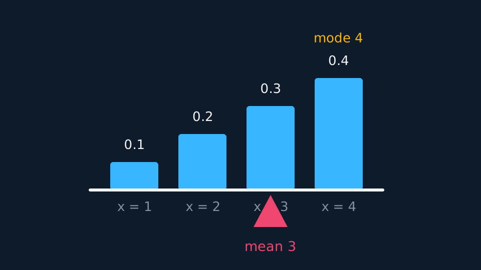
E(X) = Σ x P(X = x) is the balance point of the distribution, the value about which Σ (x − μ)P(X = x) is zero. It need not be the most probable value, and it need not be a value the variable can take at all: a fair die has mean 3.5 and no face shows 3.5. The most probable outcome is the mode.
Expectation and variance
For a discrete random variable, the expectation weights each value by its probability:
Pearson Edexcel 9FM0 formulae booklet: included, under Discrete distributions, along with E(g(X)) = Σ g(x)P(X = x). Set the values, probabilities and products out in a table before summing. E(X) is the balance point of the distribution: the value about which Σ (x − μ)P(X = x) is zero. It need not be the most probable value, and it need not be a value the variable can take. A fair die has mean 3.5 and no face shows 3.5. The mode is the most probable outcome.
WORKED EXAMPLE
A distribution, end to end
X takes values 1, 2, 3, 4 with P(X = x) = x/10. Find E(X), E(X²) and Var(X).
The probabilities 0.1, 0.2, 0.3, 0.4 sum to 1, so the model is valid.
E(X) = (1 + 4 + 9 + 16)/10 = 3.
E(X²) = (1 + 8 + 27 + 64)/10 = 10, so Var(X) = 10 − 3² = 1. The mode is 4 and the mean is 3: probability increases with x, so the mean lies below the mode.
Functions, scaling and shifting
E(g(X)) applies g to each value before weighting. So E(X²) is Σx²P(X = x), which is the sum the variance formula requires. For a linear function, E(aX + b) = aE(X) + b and Var(aX + b) = a²Var(X).
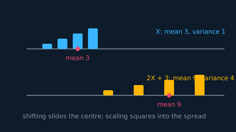
Adding b moves the mean by b and leaves the variance unchanged, because it changes every value by the same amount. Multiplying by a multiplies the variance by a², because variance is measured in squared units. Doubling every value therefore quadruples the variance and doubles the standard deviation.
WORKED EXAMPLE
Transforming the same variable
For the X above, find E(2X + 3) and Var(2X + 3).
E(2X + 3) = 2(3) + 3 = 9.
Var(2X + 3) = 2² × 1 = 4. The +3 contributes nothing to the spread.
Checking the long way, by listing the values 5, 7, 9, 11 with the same probabilities, gives the same two numbers.
Using mean and variance to assess a model
A mean and a variance can be compared with the values a named model requires. A Poisson distribution has variance equal to its mean. The theoretical binomial variance np(1 − p) is below its mean np for 0 < p < 1. A geometric distribution has variance well above its mean once p is small.
A sample mean and variance can therefore indicate whether a fitted model is plausible, but sampling variation means the comparison alone does not prove or disprove the model. In a comment on the suitability of a model, quote both calculated values, state what the proposed family requires and name the direction of any mismatch.
GUIDED PRACTICE
Judging a model
A shop models daily sales of a rare item with P(X = 0) = 0.5, P(X = 1) = 0.3, P(X = 2) = 0.2. Find the mean and variance, and comment on whether a Poisson model would fit.
Show the working
E(X) = 0 + 0.3 + 0.4 = 0.7.
E(X²) = 0 + 0.3 + 0.8 = 1.1, so Var(X) = 1.1 − 0.49 = 0.61.
The variance sits below the mean. Poisson forces the two equal, so it would overstate the day-to-day variability here.
The median of a table
The median of a discrete variable is found from the cumulative probabilities rather than by solving an equation. Run down the table adding probabilities. Under the lower-median convention, the median is the smallest value m for which F(m) ≥ 0.5. Interpolation does not apply, because the variable takes the listed values and nothing between them.
Define the median convention before using it. When the running total is exactly 0.5 at a value, the lower-median convention gives that value. Under the interval definition, every value from that one up to the next is a median, because at least half the probability lies on each side. The midpoint of the two is a third convention, matching the treatment of a data set with an even number of readings. State which convention you are using, and use the one the question specifies.
WORKED EXAMPLE
Two running totals
For X with P(X = x) = x/10 on 1, 2, 3, 4, find the median. Then find it for Y with probabilities 0.2, 0.3, 0.4, 0.1 on the same four values.
For X the running totals are 0.1, 0.3, 0.6, 1.0. The first to reach a half is at x = 3, so the median is 3 under every convention; here the mean is also 3 and the mode is 4.
For Y they are 0.2, 0.5, 0.9, 1.0, so F(2) = 0.5 exactly. The lower-median convention gives 2; the interval definition admits any value from 2 to 3; the midpoint convention gives 2.5, which is not a value Y takes. State the convention alongside the answer.
The discrete uniform, proved
A discrete uniform distribution gives each of n listed outcomes the same probability 1/n. A fair die is the standard case. The mean and variance follow in one line from the standard series sums.
For the values 1 to n, pull the constant probability out of the expectation: E(X) = (1/n)Σx = (1/n) × n(n + 1)/2. Doing the same with the squares, E(X²) = (1/n) × n(n + 1)(2n + 1)/6, which is (n + 1)(2n + 1)/6. Subtracting the square of the mean and taking a common denominator of 12 leaves (n + 1)[2(2n + 1) − 3(n + 1)]/12, and the bracket collapses to n − 1:
Both closed sums come from the compulsory series work. Pearson Edexcel 9FM0 formulae booklet: not included, so reproduce the derivation. The mean is the midpoint of the list, as the symmetry of the distribution requires, and the variance grows with the square of the number of values.
GUIDED PRACTICE
A fair die from the formulae
A fair die is rolled once. Use the two results above to write down the mean and variance of the score, and check the mean against a direct sum.
Show the working
Here n = 6, so E(X) = 7/2 = 3.5.
Var(X) = (36 − 1)/12 = 35/12 = 2.92 to three significant figures, a standard deviation of 1.71.
Directly: (1 + 2 + 3 + 4 + 5 + 6)/6 = 21/6 = 3.5, which agrees. The median is 3.5 as well, by the midpoint convention above, since the running total lands on a half at 3.
ASSESSMENT FOCUS
- Check that the probabilities sum to 1 first. Every later calculation depends on a valid distribution.
- Var(X) = E(X²) − [E(X)]². The square applies to E(X), not to the individual values.
- For Var(aX + b), state Var(aX + b) = a²Var(X) and quote the value; b does not affect the variance.
- For a median, write the running totals down the table and name the first value to reach a half.
- If a running total is exactly 0.5, name the convention you are using before giving the median.
CHECK YOURSELF
X has E(X) = 4 and Var(X) = 9. Find E(3X − 2) and Var(3X − 2).
Show a hint
Means shift and scale; variances only scale, by the square.
Show the answer
E(3X − 2) = 12 − 2 = 10. Var(3X − 2) = 9 × 9 = 81. The −2 has no effect on spread.
E(X) = Σ x P(X = x) is the balance point, and Var(X) = E(X²) − μ² measures the scatter round it.
E(aX + b) = aE(X) + b while Var(aX + b) = a²Var(X). Shifting moves the centre; scaling enters the spread squared.
The median is the first value whose running total reaches a half, and a discrete uniform on 1 to n has mean (n + 1)/2 and variance (n² − 1)/12.
WORKBOOK
Printable practice for this topic: original exam-style questions with room to work, and a fully worked answer book. Free to use; please do not redistribute or sell.
Or read them with their worked answers on the discrete random variables and expectation questions page.
USED LATER IN
CHECK YOUR PROGRESS
Rate how confident you feel with each objective for this lesson. Ratings are saved in this browser, on this device, unless you sign in.
- Check that a distribution is valid, and find an unknown constant in one by making the probabilities total 1.
- Compute E(X) and Var(X) from a probability distribution table.
- Evaluate E(g(X)) for functions such as X² and aX + b.
- Use the mean and variance to judge whether a proposed model fits observed data.
- Locate the median of a discrete distribution from its running total.
- Derive the mean and variance of a discrete uniform distribution.
- Use Var(aX + b) = a²Var(X), where the shift contributes nothing.
Open the full revision checklist to see every objective in the course in one place.