Physics › Required practicals › The inverse-square law for gamma radiation
REQUIRED PRACTICAL 12The inverse-square law for gamma radiation
Testing how the intensity of gamma radiation falls off with distance from a source, correcting for background.
Theory: Alpha, beta and gamma radiation · Radioactive decay and the decay constant
What you are trying to do
Show that the intensity of gamma radiation falls with the inverse square of distance from the source, correcting for background radiation.
Apparatus
- A sealed gamma source in its shielded holder or lead castle, handled only by the teacher with long tongs
- Geiger-Müller tube and counter, on a rule so the tube-to-source distance can be set
- A metre rule; a stopclock if the counter lacks a timer
Variables
- Independent: the measured distance x from source to tube window
- Dependent: the corrected count rate
- Control: the same source and tube, counting long enough at each distance for good statistics
Method
- With the source locked away, measure the background count over several minutes, more than once, and average to a background rate.
- With the source in place, count at each of a series of distances. Decay is random, so longer counts mean smaller fractional statistical error: count for minutes, not seconds, especially at large x where the rate is low.
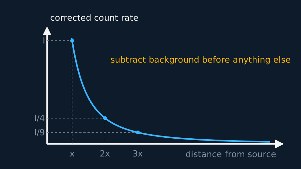
- Subtract the background from every reading before any analysis.
Analysis
- The true distance from the radiating material to the tube's sensitive volume is x plus an unknown offset: source and detector both hide their reference points inside casings.
- So do not plot C against 1/x². Instead use C = k/(x + x₀)², rearranged: 1/√C = (x + x₀)/√k. Plotting 1/√C against x gives a straight line whatever the offset; the gradient is 1/√k and the intercept is x₀/√k, so the hidden offset comes out as the intercept divided by the gradient.
- What a straight line here supports. It is evidence for the inverse-square law for gamma rays in air across the distances you counted, and the intercept divided by the gradient locates the hidden reference point inside the casings, usually a centimetre or two. The claim stops at the edges of the data. Closer in, the tube misses counts while it recovers from the last one; further out, the corrected rate is a small difference between two similar numbers. The law is being tested where the counting is good rather than everywhere.
- The limitation you cannot repeat away. Neither the source nor the tube tells you where its active volume sits, so the distance on the rule is never the distance in the equation, and that is why the plot is built to tolerate an offset rather than to assume one. The improvement that pays here is to count to a fixed number of counts rather than for a fixed time. A one-minute count gives thousands near the source and a couple of hundred far away, so the far points, which have the longest lever on the gradient, are the ones you know least well.
A worked set of readings
Counts converted to rates; background 25 counts per minute already subtracted in the third column:
| x / m | Raw rate / min⁻¹ | Corrected C / min⁻¹ | 1/√C / min½ |
|---|---|---|---|
| 0.100 | 2525 | 2500 | 0.0200 |
| 0.150 | 1271 | 1246 | 0.0283 |
| 0.200 | 769 | 744 | 0.0367 |
| 0.300 | 377 | 352 | 0.0533 |
| 0.400 | 229 | 204 | 0.0700 |
| 0.500 | 158 | 133 | 0.0867 |
Idealised illustrative data, chosen so the working is easy to follow. Real readings scatter about the line rather than sitting on it, and your own graph will have points either side of the best fit.
1/√C against x is a straight line: the inverse-square law. The gradient is 0.1667, so k = 1/gradient² = 36 counts per minute at one metre equivalent. The intercept is 0.0033, and intercept ÷ gradient = 0.0033/0.1667 places the hidden offset at x₀ = 2 cm inside the casings.
Evaluating the result
Idealised counts with one reading far off the line and two merely scattered. Decay is random, so a raw count of N carries a spread of about √N. The corrected count C in this table is not a raw count: it is the difference of two counts each measured independently over one minute, the total and the background, each with its own Poisson scatter. Variances add across a subtraction, so the spread on C is σ = √(Ntotal + Nbackground) = √(C + 2B), which with B = 25 counts per minute is √(C + 50). Rooting C alone understates it, and an understated spread makes a sound reading look like an anomaly. The question at every point is not whether a reading is off the line but whether it is off by more than the counting statistics allow.
| x / m | Corrected count C in one minute | Difference from the line | σ = √(C + 2B) |
|---|---|---|---|
| 0.200 | 766 | +22 | 29 |
| 0.300 | 335 | −17 | 20 |
| 0.400 | 311 | +107 | 19 |
Idealised illustrative data, chosen so the working is easy to follow. Real readings scatter about the line rather than sitting on it, and your own graph will have points either side of the best fit.
The first two rows are 22 and 17 counts from the line with spreads of 29 and 20, so they are not anomalies and correcting them would be inventing data. The third is 107 counts high where σ is only 19, more than five times the spread, and that needs an explanation. The candidates include another source nearby, a tube that was not at the distance recorded, and a mistimed count. Count again at that distance, and for longer, before deciding between them. Keep the original count in the table with the reason recorded, even if it is excluded from the fit.
Where the uncertainty comes from
- Counting statistics: A raw count of N carries an uncertainty of about √N, so the fractional error shrinks as counts grow; this is why the long counts are not optional. Subtracting the background does not remove that randomness; it adds a second helping of it: for two independent counts taken over equal times, the corrected count carries √(Ntotal + Nbackground), never √C.
- Background drift: Background varies; measuring it before and after and averaging is the standard guard.
- The hidden offset: The biggest systematic, and the 1/√C plot is its cure; plotting against 1/x² with the raw x would curve the line and wreck the test.
- Dead time: At very high rates a GM tube misses counts; keeping the closest distance modest sidesteps it.
What earns the marks
✓Marks
- Subtract background, and say how background was measured.
- Justify long counts from the randomness of decay: √N statistics, and combine the total and the background as √(Ntotal + Nbackground) rather than rooting the corrected count.
- The 1/√C against x plot, and why: it accommodates the unknown source and detector offsets, which plotting C against 1/x² does not.
- State the handling precautions: long tongs, maximum distance, minimum exposure time, and the source returned to its labelled storage container immediately.
Safety
!Caution
Keep the source in its shielded holder or collimator, minimise exposure time, maximise distance, and return it to its labelled storage container immediately. Never direct an unshielded or collimated beam towards a person.
Method and analysis here follow the standard approach; your school may vary the apparatus. Always follow your teacher’s risk assessment in the lab.