Radioactive decay and half-life

Random for one, dependable for a mole

Radioactive decay is random. No measurement can tell you when a given nucleus will go, and nothing you do to it, heat, pressure or chemistry, alters its chances. What each nucleus carries instead is a fixed decay constant λ, the probability of decaying per second. Model it with dice. Each die has no memory at all, yet a large enough handful loses very nearly one sixth of its number per throw.

None of that has to be taken on trust, because a counter shows it to you in a minute. Point a Geiger tube at a steady source and record the number of counts in one ten-second interval after another. The readings do not repeat: 412, then 380, then 401, then 435. Nothing about the experiment has changed between them, so every one of those differences is the randomness of individual decays showing through. Those fluctuations in count rate are the experimental evidence that decay is random. Were each nucleus keeping to a schedule, every interval would return the same number.

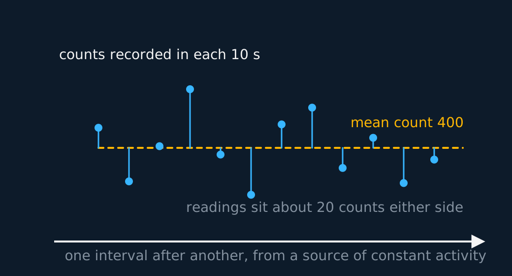
The scatter has a predictable size even though no single reading does. A count of N carries an uncertainty of about √N, so a mean of 400 scatters by about 20, one part in twenty, while a mean of 10 000 scatters by about 100, one part in a hundred. Count for longer and the fractional scatter shrinks, which is why a serious measurement counts for minutes rather than seconds. It also settles what kind of quantity an activity is. It is a statistical average from the outset, and quoting one as though it were an exact reading claims a precision the physics does not offer.

With N undecayed nuclei each carrying probability λ per second, the expected rate of loss is

and the size of that rate is the activity A, measured in becquerels, one decay per second.

Counting nuclei is chemistry's job. A mass m of a nuclide with molar mass M holds m/M moles, so N = (m/M) × N_A nuclei, with the Avogadro constant from the data booklet. Exam questions lean on this chain often.

The exponential and its half-life

A rate of loss proportional to the amount remaining is the recipe you met with capacitor discharge, and it has the same solution.

The half-life is the time for N to halve. Set N = N₀/2 and take logs. From e^-λT = 1/2 comes λT = ln 2, so

A big decay constant means a short half-life and a fierce source. Because activity is proportional to N, it decays with the same clock,

which is the form the detector actually sees. Two half-lives leave a quarter and three leave an eighth, and halving forever never reaches nothing.

Reading decay data

From a decay curve, read the half-life directly. Find the time for the activity to halve, then check it again from a different starting point, because a genuine exponential halves in the same time everywhere along its length.

For scattered data the better tool is the promised twin of the capacitor practical. Taking natural logs gives ln N = ln N₀ − λt, a straight line of ln N against t with gradient −λ. Straightness is the evidence the decay is exponential, and the gradient gives λ, from which T½ = ln 2/λ follows. Symbol for symbol, this is the RP9 analysis with λt in place of t/RC.

The half-life sets the applications. Radioactive waste must be stored securely for many half-lives of its longest-lived components, which for some isotopes means centuries. Dating runs the clock backwards. Living things hold a known fraction of carbon-14, so the fraction still left in a bone, with T½ = 5730 years, dates its death.

Running the decay forwards

ΔN/Δt = −λN is a statement about the next instant rather than about the whole decay, and a spreadsheet can march it forwards without ever solving it. Choose an interval Δt short enough that only a small fraction of the sample goes in it. Take the undecayed count at the start of the interval, work out the loss as ΔN = −λNΔt, subtract it, and repeat down the column. The exponential appears as a result rather than an assumption, and a half-life read off the modelled curve agrees with ln 2/λ.

The model carries the same built-in error as the capacitor version of it, for the same reason. Across each step the decay rate is held at the value it had at the beginning, while the real sample's rate falls throughout the step, so every step removes slightly too many nuclei and the modelled curve runs below the true exponential.

Two things the model cannot do are worth saying out loud before anyone offers a spreadsheet as evidence. It cannot fluctuate: its column is the expected count, smooth to as many decimal places as you keep, while a real sample scatters about that expectation by roughly √N. And it will report a third of a nucleus, because the arithmetic goes on working long after the physics has stopped. To check the model against the analysis, log the modelled counts and plot them against time; the line should be straight with a gradient of magnitude λ.

Which nuclei decay, and how

Plot every stable nuclide as a point with proton number Z across and neutron number N up, and they hug a narrow stable band, with N roughly equal to Z for light nuclei and bending neutron-rich as Z grows. Extra neutrons add strong-force glue without adding proton repulsion, and that is the reason for the bend.

Position on the map predicts the decay. Neutron-rich nuclei, above the band, undergo β⁻ decay, in which a neutron becomes a proton, so N falls by 1 and Z rises by 1. ⁹⁰Sr becomes ⁹⁰Y, Z climbing from 38 to 39, plus e⁻ and an antineutrino ν̅_e. Proton-rich nuclei, below the band, travel the other way by β⁺ decay or by electron capture, each turning a proton into a neutron. The heaviest nuclei shed bulk instead. In α decay, ²²⁶Ra becomes ²²²Rn with Z falling from 88 to 86, plus ⁴He, so A drops by 4 and Z by 2. In every equation, A and Z balance across the arrow.

Decay often leaves the daughter in an excited state. Nuclei have energy levels much as atoms do, drawn as nuclear energy level diagrams, and the drop to the ground state emits a γ photon. Medicine exploits one such state deliberately. Technetium-99m is a long-lived excited state that emits gamma alone, with a six hour half-life. Injected as a tracer, its photons escape the body to a camera, and within a couple of days the activity has fallen to almost nothing.