Maths › Decision Mathematics 1 › Linear programming: formulation and graphical solution
Linear programming: formulation and graphical solution
Linear programming translates a constrained problem described in words into an objective function and inequalities, and an optimal solution, when one exists, lies at a vertex of the feasible region. Formulate the problem, draw the feasible region, and locate the optimal vertex by the objective-line or vertex method.
Builds on Simultaneous equations and inequalities and Straight lines.
IN THIS TOPIC
- Define variables and write a problem as an objective and constraints.
- Shade the feasible region and find the optimum by vertex or objective line.
- Introduce slack, surplus and artificial variables correctly.
- Say over what range of a coefficient the optimal vertex survives, and what a relaxed constraint is worth.
- Deal with a problem whose variables must be whole numbers, by branch and bound where the method is named.
COMMON MISCONCEPTION
The optimal solution of a linear program is always at the vertex furthest from the origin.
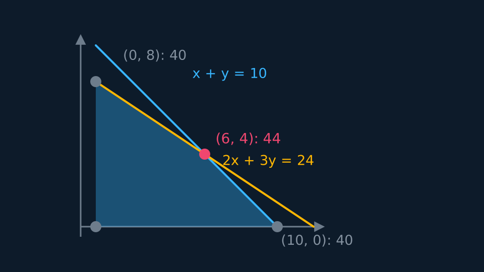
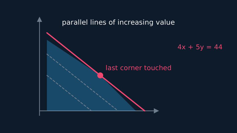
The optimum sits at a vertex of the feasible region, and which vertex is decided by the gradient of the objective, not by distance from the origin. Maximising P = 4x + 5y subject to x + y ≤ 10 and 2x + 3y ≤ 24 gives 44 at (6, 4), beating the 40 at (10, 0), which lies further out. Slide an objective line across and take the last corner it touches.
Writing the problem down
Define the variables in words, including their units. Marks are lost for an unexplained x far more often than for the algebra. Then write the objective to be maximised or minimised, and each restriction as an inequality, remembering the non-negativity conditions the context implies.
Inequalities become equations by adding a variable. A slack variable is added to a ≤ constraint to take up the unused amount. A surplus variable is subtracted from a ≥ constraint to record the excess. An artificial variable is then added to that same constraint, because subtracting the surplus leaves no starting solution to work from.
WORKED EXAMPLE
Testing the corners
Maximise P = 4x + 5y subject to x + y ≤ 10, 2x + 3y ≤ 24 and x, y ≥ 0.
The vertices are (0, 0), (10, 0), (0, 8) and the intersection of the two lines.
Solving x + y = 10 with 2x + 3y = 24 gives 30 − x = 24, so x = 6 and y = 4.
P at the four corners: 0, 40, 40 and 44. The maximum is at (6, 4), which is nearer the origin than (10, 0), so distance is not what decides it.
Two ways to find the corner
The vertex method evaluates the objective at every corner and takes the best. It is reliable and needs no judgement, and with four or five corners it is quick enough.
The objective line method draws one line of constant objective value and slides it parallel across the region, and the last corner it touches is the optimum. It is faster, and it shows at once when two corners tie, which happens when the objective runs parallel to a constraint. Whichever method you use, say which, and draw the line if the question asks for it.
When the variables must be whole numbers the optimum may not sit at a corner at all. Find the corner first, then test the integer points around it that lie inside the region, and give the best of those. Rounding the corner coordinates can land you outside the region entirely.
GUIDED PRACTICE
Slack at the optimum
For the same problem, find the value of each slack variable at the optimum and say what it means.
Show the working
At (6, 4) the first constraint gives 6 + 4 + s1 = 10, so s1 = 0.
The second gives 12 + 12 + s2 = 24, so s2 = 0.
Both slacks are zero, so both constraints are binding: the optimum sits exactly where the two lines meet.
A non-zero slack would mean spare capacity in that constraint, and relaxing it further would not improve the answer.
What a change to a coefficient does
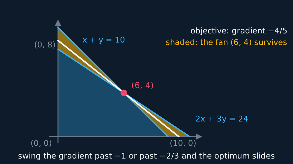
A formulation is a model, and its numbers are estimates. So a question may ask what a change to one of them would do, and the objective line answers it without any recalculation. Only the gradient of that line decides which corner it last touches, so the optimal corner survives any change to the objective that leaves the gradient between the gradients of the two constraints meeting there. Move it past either and the optimum slides to the neighbouring corner.
For the problem above, P = 4x + 5y has gradient −4/5, and the two constraints crossing at (6, 4) have gradients −1 and −2/3. Write the objective as ax + 5y and its gradient is −a/5, which sits between those two while 10/3 ≤ a ≤ 5. At a = 5 the objective runs parallel to x + y = 10 and (10, 0) ties with (6, 4); above 5 the corner (10, 0) wins outright. At a = 10/3 the tie is with (0, 8), and below that (0, 8) takes it.
Drawn on the region, the range is a fan of lines through the corner, and the answer is stable over the whole of it, not only at the one gradient the estimate happened to give.
Describe the drawing
The feasible quadrilateral for the worked problem, with its corner at six and four ringed. Three lines are drawn through that corner: the two constraint lines, of gradient minus one and minus two thirds, and between them the objective line of gradient minus four fifths. The wedge each pair of outer lines cuts out, above the corner and below it, is shaded amber: any objective whose gradient lies in that fan leaves six and four as the last corner the line touches. Tilt it past minus one and the corner at ten and nought takes over; tilt it past minus two thirds and nought and eight does.
Changing a constraint instead moves the region rather than the line. Raise the first limit from 10 to 11 and the two constraints now cross at (9, 2), where P = 46, so the extra unit was worth 2. Raise it again to 12 and the crossing is (12, 0), worth 48, the same gain once more. Past 12 the constraint stops binding, the second one alone fixes the corner, and further units are worth nothing. So the value of relaxing a constraint is constant over a range and then stops.
WORKED EXAMPLE
How far the profit can move
For the same problem, maximise P = 4x + by. Find the values of b for which (6, 4) stays optimal, and say what happens outside them.
The objective line has gradient −4/b, and it must sit between the gradients −1 and −2/3 of the two constraints through (6, 4).
So 2/3 ≤ 4/b ≤ 1, which gives 4 ≤ b ≤ 6.
Check the ends. At b = 6: P at (6, 4) is 24 + 24 = 48 and at (0, 8) it is 48 as well, so the two corners tie and above 6 the corner (0, 8) wins.
At b = 4: P at (6, 4) is 24 + 16 = 40 and at (10, 0) it is 40, another tie, and below 4 the corner (10, 0) wins.
So the answer is stable over a band rather than at a point, which is the useful thing to report: the plan at (6, 4) stands anywhere between 4 and 6, and the estimate of 5 sits comfortably inside that.
Integer programming and branch and bound
Testing the lattice points near a corner works while there are few of them. Branch and bound is the systematic version, and it is what a question naming the method wants. Solve the problem without the integer condition first; that answer is an upper bound on anything the integer problem can reach. If it happens to be whole, the work is over. If not, pick a variable with a fractional value and branch: one subproblem takes that variable at or below the value rounded down, the other at or above the value rounded up, and between them they hold every integer point of the original.
Each subproblem is then solved the same way, and its relaxed optimum is a bound on that branch. Two things end a branch. An integer answer ends it and becomes the best so far. A relaxed optimum no better than the best integer answer already found ends it as well, since nothing inside can beat what is in hand, and cutting a branch off on that ground is what stops the tree from doubling for ever.
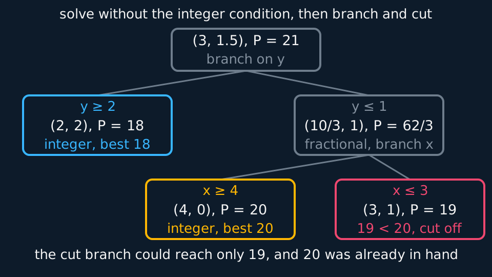
Five nodes are enough to show both endings at work, and the tree below is the one the worked example builds: each box carries the best integer answer in hand when it was reached, and the last branch cuts itself off against that figure.
Describe the drawing
A branch and bound tree of five boxes. The root solves the problem without the integer condition and reaches 21 at three and a half, so y is the variable to split on. Taking y at least two gives a whole answer straight away, (2, 2) worth 18, which becomes the best so far. Taking y at most one reaches 62 over 3, better than 18, so that branch is split again on x. With x at least four the answer is (4, 0) worth 20, whole, and the best so far rises to 20. With x at most three the branch can reach only 19, which cannot beat 20, so it is cut off and the search ends at x = 4, y = 0 with P = 20.
WORKED EXAMPLE
Branch and bound on a small problem
Maximise P = 5x + 4y subject to 6x + 4y ≤ 24 and x + 2y ≤ 6, with x and y non-negative integers.
Relaxed problem: the two constraints cross at x = 3, y = 1.5, where P = 21. That is the upper bound, and y is fractional, so branch on y.
Branch y ≥ 2: the best point of the region is (2, 2) with P = 18, and it is already whole. Record 18 as the best integer answer so far.
Branch y ≤ 1: the best point is (10/3, 1), where P = 50/3 + 4 = 62/3, a little over 20. That beats the 18 in hand, so the branch is worth splitting, and x is the fractional variable.
Branch y ≤ 1 with x ≥ 4: the constraint 6x + 4y ≤ 24 then forces y = 0 and x = 4, giving P = 20, whole. The best so far becomes 20.
Branch y ≤ 1 with x ≤ 3: the best point is (3, 1) with P = 19, which is below 20, so the branch is cut off and the search is over.
The answer is x = 4, y = 0 with P = 20. Rounding the relaxed optimum (3, 1.5) down to (3, 1) would have given 19, which is the mistake the method exists to prevent.
ASSESSMENT FOCUS
- Define every variable in words with its units before writing any inequality.
- Include the non-negativity constraints; without them the feasible region is unbounded below.
- Say which method you used, and for the objective line method draw the line.
- For integer problems, test the lattice points near the corner instead of rounding.
- Asked how far a coefficient may move, compare the objective's gradient with the gradients of the two constraints through the optimal corner.
- In branch and bound, record the best integer answer so far at every stage and say which branches it lets you cut off.
- Shade consistently and label which side of each line is allowed, or the region will be ambiguous.
CHECK YOURSELF
Write 5x + 2y ≥ 30 as an equation using a surplus and an artificial variable.
Show a hint
Subtract the surplus, then add the artificial.
Show the answer
5x + 2y − s₁ + t₁ = 30, where s₁ is the surplus recording the excess over 30 and t₁ is the artificial variable that provides a starting solution.
The optimum of a linear program sits at a vertex of the feasible region, though not necessarily the furthest one from the origin.
A ≤ constraint gains a slack variable; a ≥ constraint loses a surplus variable and gains an artificial one.
The optimal corner survives while the objective's gradient stays between the gradients of the two constraints meeting there.
Branch and bound splits on a fractional variable and cuts off any branch whose relaxed optimum falls short of the best integer answer so far.
WORKBOOK
Printable practice for this topic: original exam-style questions with room to work, and a fully worked answer book. Free to use; please do not redistribute or sell.
Or read them with their worked answers on the linear programming: formulation and graphical solution questions page.
USED LATER IN
CHECK YOUR PROGRESS
Rate how confident you feel with each objective for this lesson. Ratings are saved in this browser, on this device, unless you sign in.
- Define variables and write a problem as an objective and constraints.
- Shade the feasible region and find the optimum by vertex or objective line.
- Introduce slack, surplus and artificial variables correctly.
- Say over what range of a coefficient the optimal vertex survives, and what a relaxed constraint is worth.
- Deal with a problem whose variables must be whole numbers, by branch and bound where the method is named.
Open the full revision checklist to see every objective in the course in one place.