Maths › Exponentials and logarithms › Log graphs and exponential models
Log graphs and exponential models
Plotting log y against log x gives a straight line for a power law, and plotting log y against x gives a straight line for an exponential, with the gradient and intercept determining the constants. Fit such a model to data, use it, and state the conditions under which it stops being reasonable.
Builds on Logarithms and their laws and Straight lines.
Used in InkPhysics: The time constant and exponential decay.
IN THIS TOPIC
- Linearise y = axn and y = kbx with the right choice of log plot.
- Read the constants of a model off a log graph's gradient and intercept.
- Interpret, use and criticise exponential growth and decay models.
COMMON MISCONCEPTION
A straight line on a log graph means the data is linear.
The straight line is on logarithmic axes, so the relationship between x and y is not linear. A line on log y against log x indicates a power law y = axn, with gradient n and intercept log a; a line on log y against x indicates an exponential y = kbx, with gradient log b and intercept log k. The plot that straightens the data identifies the family.
Two shapes, two log plots
Taking logarithms of a power law y = axn, for x > 0 and a > 0, gives log y = log a + n log x. Plot log y against log x and that is a straight line, gradient n and intercept log a. Take logs of an exponential y = kbx instead and you get log y = log k + x log b, a straight line when log y is plotted against x itself. Whichever plot gives a straight line identifies the model that fits the data.
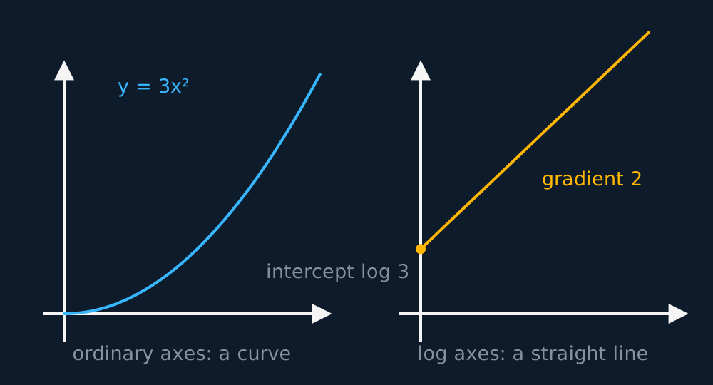
The straight line is on logarithmic axes, so the relationship between x and y is not linear; a straight line on those axes is evidence of a power law or an exponential relationship.
WORKED EXAMPLE
Constants from a log-log line
A quantity follows y = axn, and measurements give (2, 12) and (5, 75). Find n and a.
The gradient of the log-log line is n = (log 75 − log 12)/(log 5 − log 2) = 0.7959/0.3979 = 2.
Then log a = log 12 − 2 log 2 = log 3, so a = 3, and the law is y = 3x2.
Use any third data point to check the fitted model: here 3 × 42 = 48 would confirm a reading at (4, 48).
GUIDED PRACTICE
Constants from a log-linear line
Plotting log10 y against x gives a straight line with intercept 0.30 and gradient 0.15. Find the model in the form y = kbx, before opening the working.
Show the working
The intercept is log k, so k = 100.30 = 2.0 to 2 significant figures.
The gradient is log b, so b = 100.15 = 1.41.
The model is y ≈ 2.0 × 1.41x, an increase of about 41% per unit of x. The intercept is log k rather than k, so it must be un-logged.
Decay, half-life and the long run
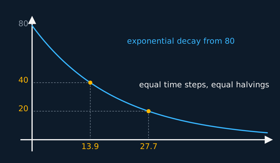
Exponential decay is the same model with a negative constant, m = Ae−kt with k > 0. Equal time intervals multiply the quantity by equal factors, so the time taken to halve is the same from any starting point on the curve.
WORKED EXAMPLE
A decay model, read in full
A mass in grams is modelled by m = 80e−0.05t, t in days. State the initial mass, find m after 10 days, and find how long the mass takes to halve.
At t = 0 the mass is the front constant, 80 g.
m(10) = 80e−0.5 = 48.5 g.
Halving needs e−0.05t = ½, so t = ln 2/0.05 = 13.9 days, and the same 13.9 days halves it again after that.
INDEPENDENT PRACTICE
Where the model breaks
A bacteria population is modelled by P = 2000e0.1t, t in hours. Evaluate the model's prediction at t = 100, and explain why the model must fail long before then.
Show the working
P(100) = 2000e10 ≈ 4.4 × 10⁷, twenty-two thousand times the starting population.
The model assumes the growth rate remains proportional to P for all t. In a real colony, food, space and the accumulation of waste limit the population, so the assumption fails above some size.
A complete answer names the assumption, names the limiting resource, and proposes a specific refinement, such as a model whose growth rate decreases as P approaches a limiting value.
ASSESSMENT FOCUS
- Choose the plot to match the proposed model: log y against log x for a power law, log y against x for an exponential, and state which has been chosen.
- The gradient and intercept of the logarithmic plot are n and log a for a power law, or log b and log k for an exponential. Un-log the intercept before quoting the constant.
- A half-life question reduces to e−kt = ½, so t = ln 2/k.
- “Initial” means the value at t = 0, where the exponential factor is 1 and the value is the constant A.
CHECK YOURSELF
The model y = 4 × 2x is to be drawn as a straight line. State what should be plotted, and give the line's gradient and intercept.
Show a hint
Take log base 10 of both sides and read the structure.
Show the answer
Taking logs gives log y = log 4 + x log 2, so plot log y against x.
The gradient is log 2 ≈ 0.301 and the intercept is log 4 ≈ 0.602.
The intercept is twice the gradient because 4 = 22, which checks the two values.
A power law gives a straight line on log-log axes and an exponential gives one on log-linear axes; the plot that straightens the data identifies the model.
In Aekt, A is the value at t = 0, k is the proportional rate of change, and ln 2 divided by |k| is the doubling or halving time.
WORKBOOK
Printable practice for this topic: original exam-style questions with room to work, and a fully worked answer book. Free to use; please do not redistribute or sell.
Or read them with their worked answers on the log graphs and exponential models questions page.
USED LATER IN
CHECK YOUR PROGRESS
Rate how confident you feel with each objective for this lesson. Ratings are saved in this browser, on this device, unless you sign in.
- Linearise y = axn and y = kbx with the right choice of log plot.
- Read the constants of a model off a log graph's gradient and intercept.
- Interpret, use and criticise exponential growth and decay models.
Open the full revision checklist to see every objective in the course in one place.