Maths › Further Pure 1 › Numerical methods for differential equations
Numerical methods for differential equations
A finite-difference formula replaces a derivative by values on a grid. State the step length, use consistent indexing and retain sufficient precision between steps. Give the approximation order only with the required smoothness assumptions, and compare methods by the errors they actually produce.
Builds on Locating roots and iteration and Second order equations.
IN THIS TOPIC
- Quote and apply the forward and central difference formulae for dy/dx.
- Step a first or second order equation forward with a stated step length h.
- Apply Simpson's rule with an even number of strips and compare its estimate with an exact value.
- Apply the mid-ordinate rule, and say which way its error runs against that of the trapezium rule, with the assumptions that comparison needs.
COMMON MISCONCEPTION
A differential equation with no closed-form solution cannot be evaluated at a particular point.
A difference formula turns the equation into a rule for the next value, so a solution with no closed form can still be tabulated. The forward difference rearranges to give yn+1 from yn and the gradient the equation supplies; the central difference uses a step each side and, for a smooth function and small h, has truncation error of order h² against order h.
Derivatives as differences
Over a short step h, a derivative is nearly a gradient between two sampled points. Two approximations for the first derivative carry most of this topic.
Check the current formula booklet for your awarding organisation; whether or not the difference formulae are supplied, you must know when each applies. The first is the forward difference, which uses the step ahead. The second is the central difference, which uses a step each side of the point. For sufficiently smooth functions and small equal step length, central differences have local truncation error of order h², compared with order h for a forward difference. Rearranging either for yn+1 gives a rule for the next value, so a solution with no closed form can still be tabulated.
WORKED EXAMPLE
Two steps, two methods
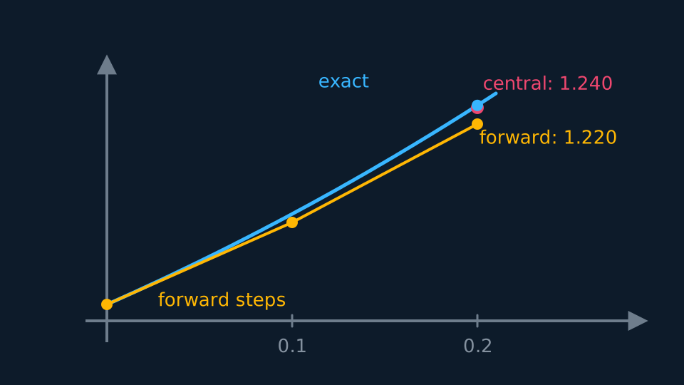
For dy/dx = x + y with y = 1 at x = 0 and h = 0.1, estimate y at x = 0.2.
Forward difference: y₁ = 1 + 0.1(0 + 1) = 1.1, then y₂ = 1.1 + 0.1(0.1 + 1.1) = 1.22.
Central difference from x = 0.1: y₂ = y₀ + 2h(x₁ + y₁) = 1 + 0.2(1.2) = 1.24.
The exact solution 2e0.2 − 1.2 is 1.2428, so the central difference is out by 0.0028 where the forward difference is out by 0.0228, a factor of about eight on this problem at this step length.
Second order equations
The second derivative gets its own approximation, (yn+1 − 2yn + yn-1)/h², which is the central difference applied twice. Substitute it into the equation, rearrange for yn+1, and you have a recurrence that reaches back two steps instead of one.
This recurrence needs two consecutive grid values. An initial-value problem may instead give y and y′ at one point, in which case a separate starting approximation is needed to obtain the second grid value: a Taylor step y₁ ≈ y₀ + hy′₀ + ½h²y″₀ is the usual choice, with y″₀ read from the equation. A boundary-value problem giving y at each end of the interval is a third case, solved as a system rather than by stepping. Lay the values out in a table with columns for x, y and whatever the equation needs.
The mid-ordinate rule
Two of the three rules for estimating an integral share a slicing and differ only in where they sample. Cut the interval from a to b into n strips of width h. The trapezium rule reads the ordinate at each strip edge and joins consecutive pairs with a chord. The mid-ordinate rule leaves the edges alone and reads the value at the middle of each strip instead, roofing the strip with a horizontal line at that height.
So the estimate is M = h(m1 + m2 + … + mn), with mr the value of y at the centre of the rth strip. There are n mid-ordinates to n strips rather than n + 1, no weights and no end terms, so it needs the fewest evaluations of the three rules. Check the current formula booklet for your awarding organisation, since provision of the mid-ordinate and Simpson formulae differs between organisations.
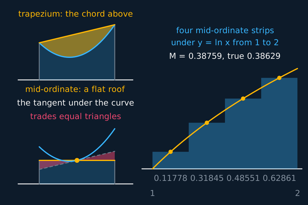
The directions of the two errors can be compared on one strip. Replace the horizontal roof by the tangent to the curve at the mid-ordinate, which encloses the same area, since the two triangles it exchanges either side of the centre are congruent. Where the curve is concave up, that tangent lies below it across the strip, so the mid-ordinate estimate is too small, while the chord of the trapezium rule lies above and its estimate is too large. A concave-down curve reverses both.
So for a twice-differentiable function whose second derivative keeps one sign across the interval, the two rules straddle the true value, and as h tends to zero the mid-ordinate error tends to half the trapezium error in magnitude. Where the concavity changes sign, the strips contribute errors of both signs and neither conclusion follows.
The left of the figure is that argument on one strip; the right is the estimate the worked example makes.
Describe the drawing
Two panels. On the left, one strip under a curve that bends upwards, drawn twice: above, the trapezium chord stands clear of the curve and the amber sliver it adds is the trapezium rule's overshoot; below, the flat mid-ordinate roof carries the dashed tangent through the centre, and the two coral triangles the tangent trades either side are congruent, so the tangent trapezium and the rectangle have the same area while the tangent itself stays under the curve. On the right, four mid-ordinate rectangles under y = ln x from 1 to 2, each roofed at the height read at its own centre, giving M = 0.38759.
WORKED EXAMPLE
One integral, two rules, opposite errors
Estimate ∫12 ln x dx with four strips by the mid-ordinate rule, and compare it with the trapezium estimate and with the exact value.
h = 0.25, so the strip centres are 1.125, 1.375, 1.625 and 1.875, and the mid-ordinates there are 0.11778, 0.31845, 0.48551 and 0.62861.
Adding those and multiplying by h: M = 0.25 × 1.55035 = 0.38759.
The trapezium rule on the same four strips gives 0.38370, and the exact value is 2 ln 2 − 1 = 0.38629. The logarithm is concave down throughout [1, 2], so by the tangent argument the trapezium estimate is too small and the mid-ordinate estimate too large.
The mid-ordinate error is +0.00129 and the trapezium error −0.00259: opposite in sign, with the trapezium error about twice the size, as the fixed concavity predicts.
Simpson's rule
Where the trapezium rule joins sample points with straight lines, Simpson's rule threads a parabola through each consecutive triple of points, so the strips must come in pairs.
Check the current formula booklet for your awarding organisation; whether or not Simpson's rule is supplied, you must know when it applies. Check the 1, 4, 2, 4, …, 4, 1 pattern of weights before evaluating anything: ends weighted 1, odd-indexed points weighted 4, even-indexed interior points weighted 2. An odd number of strips leaves a final strip with no partner, so the rule does not apply.
WORKED EXAMPLE
π/4 from four strips
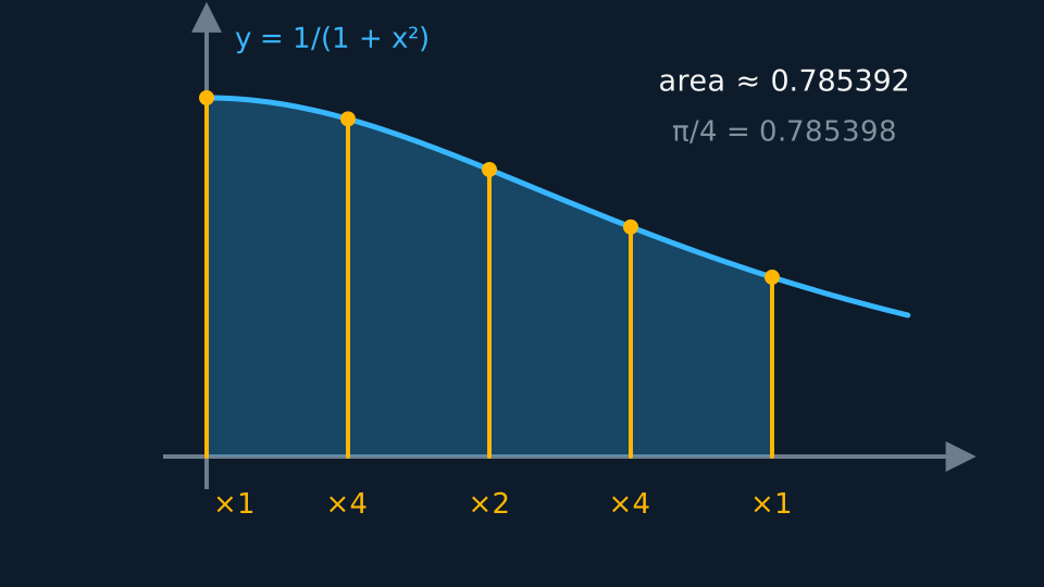
Use Simpson's rule with four strips to estimate ∫1/(1 + x²) dx from 0 to 1.
h = 0.25 and the five ordinates are 1, 0.941176, 0.8, 0.64, 0.5.
Weighted sum: 1 + 4(0.941176) + 2(0.8) + 4(0.64) + 0.5 = 9.424706.
Multiply by h/3 to get 0.785392, compared with π/4 ≈ 0.785398; the values agree to four decimal places and the absolute error is about 6 × 10⁻⁶.
The three rules are related by an identity. Run the mid-ordinate rule and the trapezium rule on the same n strips: (2M + T)/3 is the Simpson estimate on 2n strips, because halving the strip width turns each mid-ordinate into an ordinate. On the logarithm of the section before, M = 0.38759 and T = 0.38370 give 0.38629, which is Simpson's rule on eight strips to five decimal places. The weights 4 and 2 combine the two one-sided estimates in the ratio 2 : 1, which is the ratio in which their leading errors cancel.
GUIDED PRACTICE
One step of a second order equation
For y'' = x − y with y = 2 at x = 0 and y = 2.1 at x = 0.1, use the central second-difference approximation with h = 0.1 to estimate y at x = 0.2.
Show the working
The approximation gives (y₂ − 2y₁ + y₀)/h² = x₁ − y₁.
So y₂ = 2y₁ − y₀ + h²(x₁ − y₁) = 4.2 − 2 + 0.01(0.1 − 2.1).
y₂ = 2.2 − 0.02 = 2.18. The recurrence needs two consecutive grid values, which is why the question supplied y at x = 0 and at x = 0.1.
ASSESSMENT FOCUS
- State which difference formula you are using before substituting into it.
- Work to more decimal places than the answer demands, then round once at the end.
- Simpson's rule needs an even number of strips; an odd number means the strips cannot be paired.
- The mid-ordinate rule wants n heights to n strips, read at the centres, where the trapezium rule wants n + 1 read at the edges.
- Asked to compare the mid-ordinate and trapezium estimates, state the sign of the second derivative across the interval first. Where it keeps one sign, the two estimates lie either side of the true value.
- Lay the arithmetic out as a table of x and y values, so that each substitution can be checked against the one before it.
- Asked which approximation is the more accurate, give the truncation order and the smoothness assumption it needs, or compare the two errors against a known exact value.
CHECK YOURSELF
Using the forward difference with h = 0.2, take one step of dy/dx = y − x from y = 1 at x = 0.
Show a hint
y₁ = y₀ + h × (dy/dx at the start).
Show the answer
The gradient at the start is 1 − 0 = 1, so y₁ = 1 + 0.2 = 1.2 at x = 0.2. The forward difference uses only the gradient at the left-hand end of the step.
The forward difference uses the step ahead; the central difference uses a step each side and, for a sufficiently smooth function and small h, has truncation error of order h² against order h.
Second order equations use (yn+1 − 2yn + yn-1)/h², which needs two consecutive grid values; y and y′ at one point give only one, so the second is found from a starting approximation.
Simpson: h/3 with weights 1, 4, 2, …, 4, 1, and an even number of strips.
Mid-ordinate: h times the n centre heights. Where the second derivative keeps one sign across the interval, its error is opposite in sign to the trapezium rule's and, as h tends to zero, about half the size.
WORKBOOK
Printable practice for this topic: original exam-style questions with room to work, and a fully worked answer book. Free to use; please do not redistribute or sell.
Or read them with their worked answers on the numerical methods for differential equations questions page.
CHECK YOUR PROGRESS
Rate how confident you feel with each objective for this lesson. Ratings are saved in this browser, on this device, unless you sign in.
- Quote and apply the forward and central difference formulae for dy/dx.
- Step a first or second order equation forward with a stated step length h.
- Apply Simpson's rule with an even number of strips and compare its estimate with an exact value.
- Apply the mid-ordinate rule, and say which way its error runs against that of the trapezium rule, with the assumptions that comparison needs.
Open the full revision checklist to see every objective in the course in one place.