Maths › Further Pure 2 › Diagonalisation and the Cayley-Hamilton theorem
Diagonalisation and the Cayley-Hamilton theorem
A matrix is diagonalisable only when it has a full basis of independent eigenvectors. In that case M = PDP⁻¹, which simplifies powers. The Cayley-Hamilton theorem applies to every square matrix and can reduce high powers; it gives an inverse formula only when the matrix is non-singular.
Builds on Eigenvalues and eigenvectors and Determinants and inverses.
IN THIS TOPIC
- Test whether an n × n matrix has n independent eigenvectors, and build P and D when it has.
- Use diagonalisation to compute high powers of a matrix.
- Diagonalise a real symmetric matrix orthogonally, with P⁻¹ equal to the transpose.
- Apply the Cayley-Hamilton theorem to reduce powers, and to find an inverse when the matrix is non-singular.
COMMON MISCONCEPTION
Every square matrix can be written as PDP⁻¹ with D diagonal.
Only a matrix with a full set of independent eigenvectors can be written that way. An n × n matrix is diagonalisable exactly when it has n linearly independent eigenvectors, which is what makes P invertible. Distinct eigenvalues guarantee that; a repeated eigenvalue does so only when its eigenspace has dimension equal to its multiplicity, which is why a shear cannot be diagonalised.
New axes, diagonal matrix
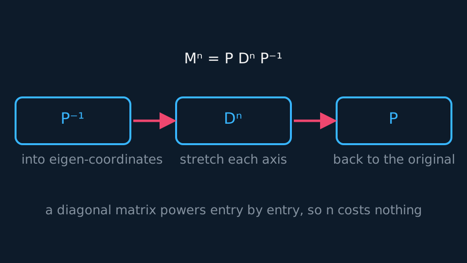
If an n × n matrix has n linearly independent eigenvectors, place them as the columns of P and put the corresponding eigenvalues in D; then M = PDP⁻¹ and Mk = PDkP⁻¹. Written the other way round, the same statement is
and it holds exactly when the columns of P are n independent eigenvectors, which is what makes P invertible. n distinct eigenvalues guarantee independence; a repeated eigenvalue does so only when its eigenspace has dimension equal to its multiplicity, which is why a shear, whose repeated eigenvalue leaves one direction only, cannot be diagonalised.
In eigenvector coordinates the transformation is a stretch along each axis and nothing more, so a diagonal matrix takes its power entry by entry and Mk costs two multiplications whatever k is.
WORKED EXAMPLE
A tenth power without ten multiplications
For the matrix with rows (4, 1) and (2, 3), describe how to find M¹⁰.
The eigenvalues are 5 and 2, with eigenvectors (1, 1) and (1, −2), so P has columns (1, 1) and (1, −2), and D is diagonal with entries 5 and 2.
D¹⁰ is diagonal with 5¹⁰ = 9765625 and 2¹⁰ = 1024.
M¹⁰ = PD¹⁰P⁻¹, which is two multiplications and a pair of powers. The two eigenvectors are independent because the eigenvalues differ, so the matrix is diagonalisable. Since 5¹⁰ is far larger than 2¹⁰, at large powers the matrix acts approximately as a stretch along y = x.
A real symmetric matrix always has an orthonormal set of eigenvectors, so it is always diagonalisable and P can be built orthogonal, making P⁻¹ the transpose of P. Eigenvectors belonging to different eigenvalues are already perpendicular and need only normalising. A repeated eigenvalue needs care, since its eigenvectors fill a whole subspace and two chosen from it need not be perpendicular: choose a perpendicular pair there, by Gram-Schmidt if the obvious choice is not perpendicular, and normalise those. The construction is called orthogonal diagonalisation.
Every matrix solves its own equation
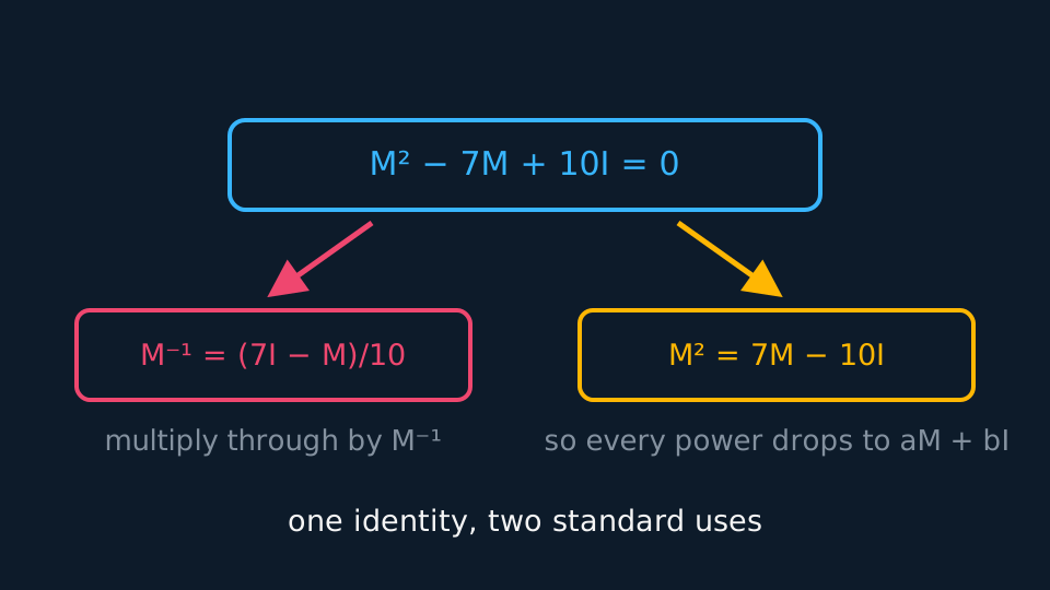
The Cayley-Hamilton theorem says that every square matrix satisfies its own characteristic equation, whether or not it is diagonalisable. For a 2 × 2 with trace t and determinant d, that reads M² − tM + dI = 0. Rearranging expresses M² in terms of M and I, so every higher power reduces to a combination of the two.
WORKED EXAMPLE
Two uses of one identity
For the matrix with rows (4, 1) and (2, 3), verify Cayley-Hamilton and use it to find M⁻¹.
M² has rows (18, 7) and (14, 11). Then M² − 7M + 10I has rows (18 − 28 + 10, 7 − 7) and (14 − 14, 11 − 21 + 10), which is the zero matrix, as promised.
Multiply the identity by M⁻¹, which exists because det M = 10 ≠ 0: M − 7I + 10M⁻¹ = 0, so M⁻¹ = (7I − M)/10, which is one tenth of the matrix with rows (3, −1) and (−2, 4).
Multiplying M by that returns the identity. The inverse came out of the characteristic equation without computing an adjugate. The step requires det M ≠ 0: for a singular matrix the constant term of the characteristic polynomial is zero and no inverse can be extracted this way.
GUIDED PRACTICE
Reducing a cube
A 2 × 2 matrix has trace 5 and determinant 6. Use Cayley-Hamilton to express M³ in terms of M and I.
Show the working
The theorem gives M² = 5M − 6I.
Multiplying by M: M³ = 5M² − 6M = 5(5M − 6I) − 6M = 19M − 30I.
For a 2 × 2 matrix every power reduces to aM + bI for some numbers a and b, however large the exponent.
ASSESSMENT FOCUS
- Say that the matrix has a full set of independent eigenvectors before writing P⁻¹MP = D; a matrix without one is not diagonalisable.
- State P and D explicitly, with the eigenvector order matching the eigenvalue order, since a mismatch makes every later line wrong.
- For real symmetric matrices, make the eigenvectors perpendicular first and then normalise, so P is orthogonal and the inverse is the transpose.
- Quote Cayley-Hamilton by name, and show the characteristic equation it comes from.
- To get an inverse from the theorem, state that the determinant is non-zero, then multiply the identity through by M inverse and rearrange.
CHECK YOURSELF
A 2 × 2 matrix M has trace 6 and determinant 5. Write down the equation Cayley-Hamilton gives, and hence M⁻¹ in terms of M and I.
Show a hint
The characteristic equation is λ² − 6λ + 5 = 0.
Show the answer
M² − 6M + 5I = 0. The determinant 5 is non-zero, so M⁻¹ exists; multiplying by M⁻¹ gives M − 6I + 5M⁻¹ = 0, so M⁻¹ = (6I − M)/5.
If an n × n matrix has n independent eigenvectors, P from the eigenvectors and D from the eigenvalues give P⁻¹MP = D and Mⁿ = PDⁿP⁻¹; without a full eigenvector basis the matrix is not diagonalisable.
For a real symmetric matrix, an orthonormal set of eigenvectors makes P orthogonal, so P⁻¹ is the transpose.
Cayley-Hamilton applies to every square matrix and reduces high powers; it yields an inverse only when the determinant is non-zero.
WORKBOOK
Printable practice for this topic: original exam-style questions with room to work, and a fully worked answer book. Free to use; please do not redistribute or sell.
Or read them with their worked answers on the diagonalisation and the Cayley-Hamilton theorem questions page.
CHECK YOUR PROGRESS
Rate how confident you feel with each objective for this lesson. Ratings are saved in this browser, on this device, unless you sign in.
- Test whether an n × n matrix has n independent eigenvectors, and build P and D when it has.
- Use diagonalisation to compute high powers of a matrix.
- Diagonalise a real symmetric matrix orthogonally, with P⁻¹ equal to the transpose.
- Apply the Cayley-Hamilton theorem to reduce powers, and to find an inverse when the matrix is non-singular.
Open the full revision checklist to see every objective in the course in one place.