Maths › Further Statistics 1 › Geometric and negative binomial distributions
Geometric and negative binomial distributions
The geometric and negative binomial distributions count the trials needed to reach a fixed number of successes. They reverse the binomial's question: the number of successes is fixed and the number of trials is random.
Builds on The Poisson distribution and Geometric series.
IN THIS TOPIC
- Model the trial of a first success with the geometric distribution.
- Extend to the rth success with the negative binomial distribution.
- Quote and apply the means and variances of both.
COMMON MISCONCEPTION
Waiting for a success is just the binomial distribution read backwards, so the same formulae apply.
It is a different family, not a rearrangement. The binomial fixes the number of trials and counts successes; the geometric fixes the successes at one and counts trials, so P(X = x) = p(1 − p)x-1 with mean 1/p and variance (1 − p)/p². Trials are still independent with constant p, but X now has no upper limit.
Waiting for the first success
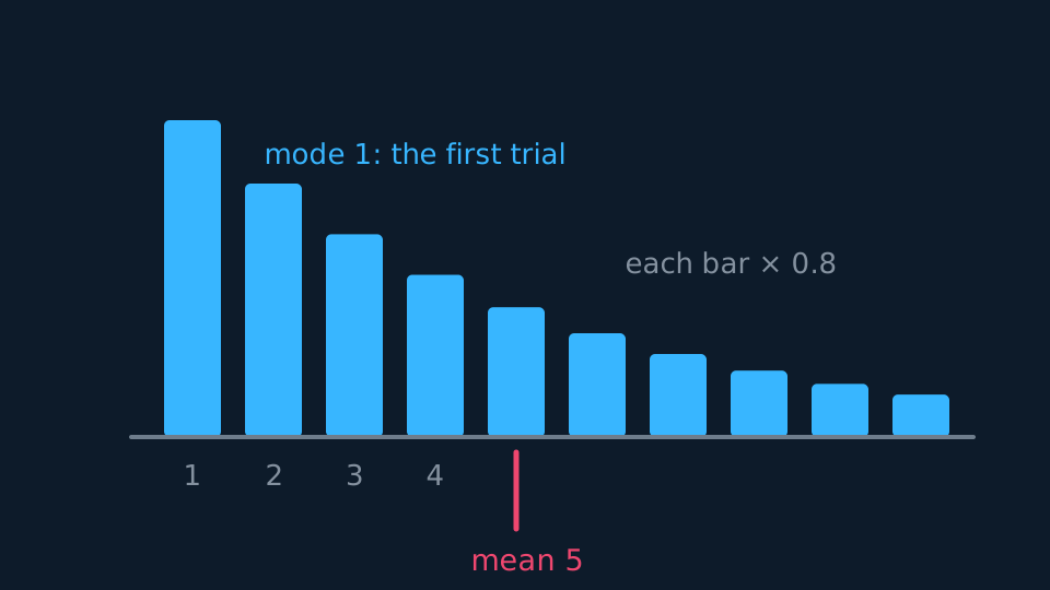
The geometric distribution used here counts the trial on which the first success arrives, so X takes the values 1, 2, 3, …; it does not count the failures before that success. A first success on trial x needs x − 1 failures then a success, so P(X = x) = p(1 − p)x-1. The binomial fixes the number of trials and counts successes; the geometric fixes the number of successes at one and counts trials, so it is a different family rather than a rearrangement of the binomial formula. Trials must still be independent with a constant p, but X now has no upper limit, and the probabilities decay geometrically, which is the origin of the name.
Pearson Edexcel 9FM0 formulae booklet: included, as one row of the table of standard discrete distributions, with the probability function, mean and variance together. Check the support convention each board or question uses before quoting a mean.
WORKED EXAMPLE
A first success
A spinner lands on red with probability 0.2. Find the probability the first red is on the third spin, and the mean number of spins needed.
P(X = 3) = 0.2 × 0.8² = 0.128.
μ = 1/p = 5 spins, with variance 0.8/0.04 = 20.
The mode is always 1, however small p is. The single likeliest trial for a first success is the first one, even when the average wait is long.
Waiting for the rth success
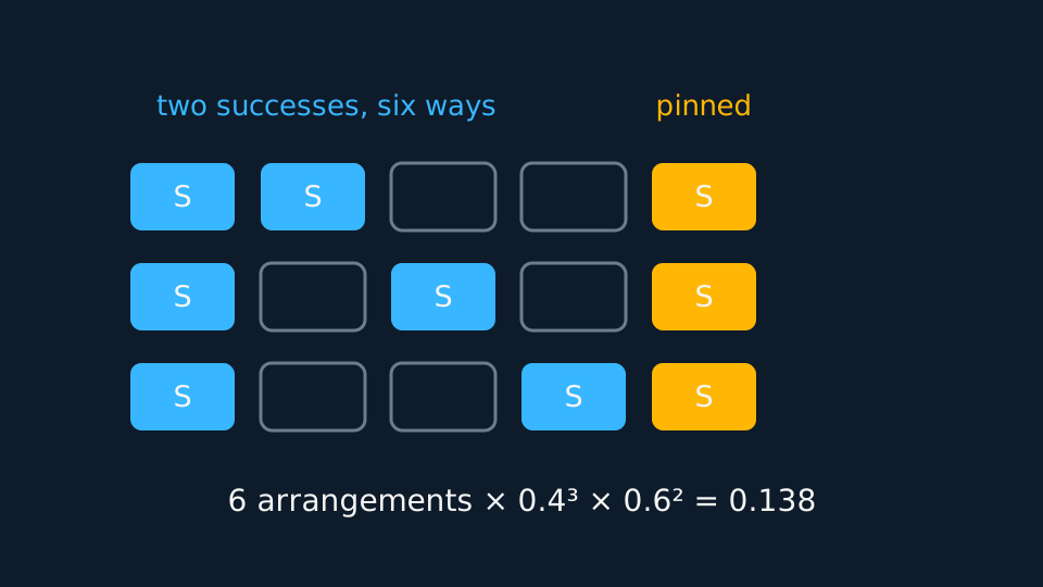
The negative binomial generalises it. For the rth success to land on trial x, the first x − 1 trials must hold exactly r − 1 successes, and trial x must succeed:
Pearson Edexcel 9FM0 formulae booklet: included, as a further row of the same table. Identifying which distribution a context describes is the part the booklet cannot supply. Here X again counts trials, not failures. The combination counts the arrangements of the earlier r − 1 successes among the first x − 1 trials; the final trial is fixed as a success and is not one of the arrangements. Setting r = 1 recovers the geometric distribution exactly, means and variances included.
WORKED EXAMPLE
The third success
Trials succeed independently with probability 0.4. Find the probability the third success occurs on the fifth trial, and the mean number of trials for three successes.
P(X = 5) = ⁴C₂ × 0.4³ × 0.6² = 6 × 0.064 × 0.36 = 0.138.
μ = r/p = 3/0.4 = 7.5 trials, with variance 3 × 0.6/0.16 = 11.25.
The mean is three times the geometric distribution's mean, because the wait for three successes is the sum of three independent geometric waits.
GUIDED PRACTICE
Recognising the model
A quality inspector tests items until finding the second faulty one. Faults occur independently with probability 0.1. Find the probability this happens on the fifth item tested.
Show the working
This is negative binomial with r = 2 and p = 0.1.
P(X = 5) = ⁴C₁ × 0.1² × 0.9³ = 4 × 0.01 × 0.729.
= 0.0292. The combination counts the four places the first fault could have taken among the earlier trials.
ASSESSMENT FOCUS
- Read what is being counted. Trials until a success is geometric or negative binomial; successes in n trials is binomial.
- State whether X counts trials or failures before quoting a mean, because the two conventions differ by 1.
- The last trial is a success in both models, so the combination only arranges the earlier ones.
- For 'at least x trials', use (1 − p) to the power x − 1. No summation is needed.
- Quote the means and variances from the formulae unless a derivation is asked for.
CHECK YOURSELF
A biased coin shows heads with probability 0.25. Find the probability that the first head appears on the fourth toss, and the mean number of tosses required.
Show a hint
Geometric with p = 0.25.
Show the answer
P(X = 4) = 0.25 × 0.75³ = 0.105. The mean is 1/0.25 = 4 tosses.
Geometric: P(X = x) = p(1 − p)x-1, mean 1/p, variance (1 − p)/p².
Negative binomial for the rth success: the combination arranges the earlier successes, and the mean is r/p.
WORKBOOK
Printable practice for this topic: original exam-style questions with room to work, and a fully worked answer book. Free to use; please do not redistribute or sell.
Or read them with their worked answers on the geometric and negative binomial distributions questions page.
USED LATER IN
CHECK YOUR PROGRESS
Rate how confident you feel with each objective for this lesson. Ratings are saved in this browser, on this device, unless you sign in.
- Model the trial of a first success with the geometric distribution.
- Extend to the rth success with the negative binomial distribution.
- Quote and apply the means and variances of both.
Open the full revision checklist to see every objective in the course in one place.