Maths › Further Statistics 1 › The Poisson distribution
The Poisson distribution
The Poisson distribution models counts of events that occur singly, independently and at a constant average rate in a fixed interval. Its single parameter λ is both the mean and the variance. Calculate Poisson probabilities, check the conditions against a context, pool independent counts, and approximate a binomial distribution.
Builds on The binomial distribution and Discrete random variables and expectation.
IN THIS TOPIC
- Model random events with Po(λ) and compute probabilities on a calculator.
- State the conditions a Poisson model requires and check them against a context.
- Use E(X) = Var(X) = λ, scale λ with the length of the window, and add independent counts.
- Approximate B(n, p) by Po(np) when n is large and p is small.
COMMON MISCONCEPTION
The Poisson distribution needs both a number of trials and a probability, just as the binomial does.
Poisson carries one parameter, the mean rate λ over the interval, which is also its variance. It counts events landing at random in a fixed interval of time or space with no upper limit on the count, and asks only that events occur singly, independently and at a constant average rate. Scaling the window scales λ with it.
Poisson probabilities, mean and variance
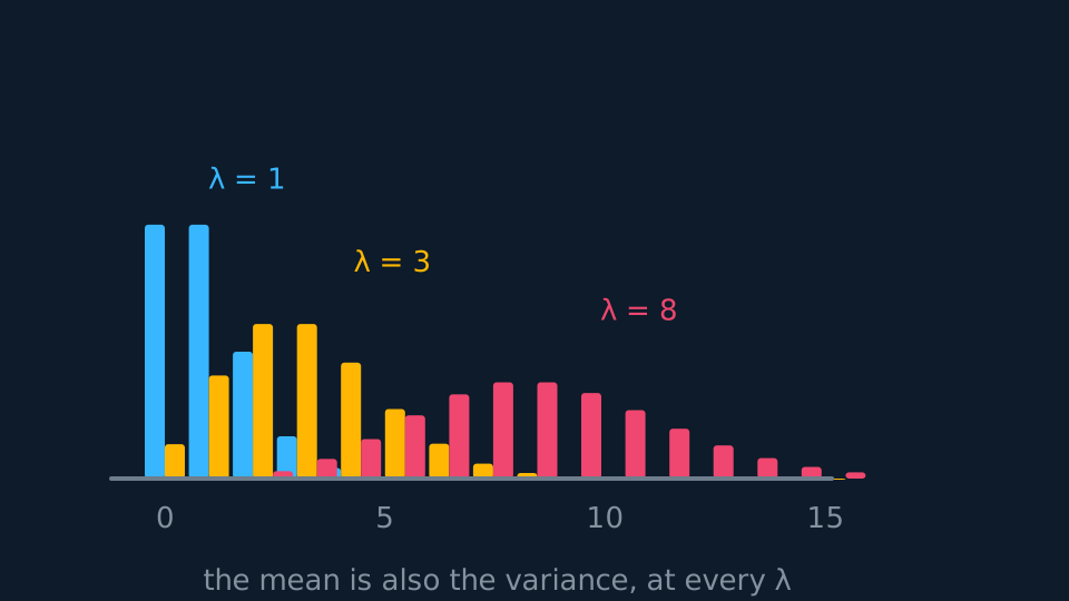
The Poisson distribution counts events landing at random in a fixed interval of time or space, with no upper limit on the count. It has no number of trials and no probability of success: the mean rate λ over the interval is the only parameter, and it is also the variance.
Pearson Edexcel 9FM0 formulae booklet: included, in the table of standard discrete distributions, with the probability function, mean and variance together. Scaling the window scales λ with it. If calls arrive at Po(3) per minute, then over five minutes they arrive at Po(15). The same additivity lets independent Poisson counts be pooled, so Po(λ) plus Po(μ) is Po(λ + μ).
WORKED EXAMPLE
Probabilities from a rate
Faults occur in a cable at a mean rate of 3 per kilometre, at random. Find the probability of exactly 2 faults in a kilometre, and of at most 1.
X ~ Po(3), so P(X = 2) = e⁻³ × 3²/2! = 0.224.
P(X ≤ 1) = e⁻³(1 + 3) = 0.199.
The mean and the variance are both 3. Every Poisson distribution has that equality, and it is the first property to compare with data.
Conditions for a Poisson model
Three conditions are required before writing Po(λ). Events must occur singly, so no two arrive at exactly the same instant. They must occur independently, so one event neither makes another more nor less likely. And they must occur at a constant average rate across the interval.
Contexts often violate one of them. Goals in football cluster because a team that scores changes how both sides play. Calls to a helpline peak at nine in the morning, so the rate is not constant over a day. In a suitability comment, name the condition you doubt and explain how the context may violate it.
The binomial distribution requires a fixed number of trials, two outcomes per trial, independent trials, and a constant probability of success. Its mean is np and its variance np(1 − p), so the theoretical variance is below the mean for 0 < p < 1. A sample variance above its mean is therefore inconsistent with a binomial model, and a sample variance well below its mean is inconsistent with a Poisson model, in both cases subject to sampling variation.
WORKED EXAMPLE
Is the model reasonable?
A garage records the number of customers arriving each hour between 8am and 6pm. Over 200 hours the mean is 6.1 and the variance 9.8. Comment on a Poisson model.
Poisson demands equal mean and variance. Here the variance is roughly 1.6 times the mean, so the counts vary more than the model allows.
The condition most likely to fail is the constant rate. Lunchtime and the end of the working day are busier than mid-morning, so pooling all ten hours mixes several rates together.
A Poisson model fitted hour by hour, or restricted to a quiet band of the day, would be more defensible.
Poisson approximation to the binomial
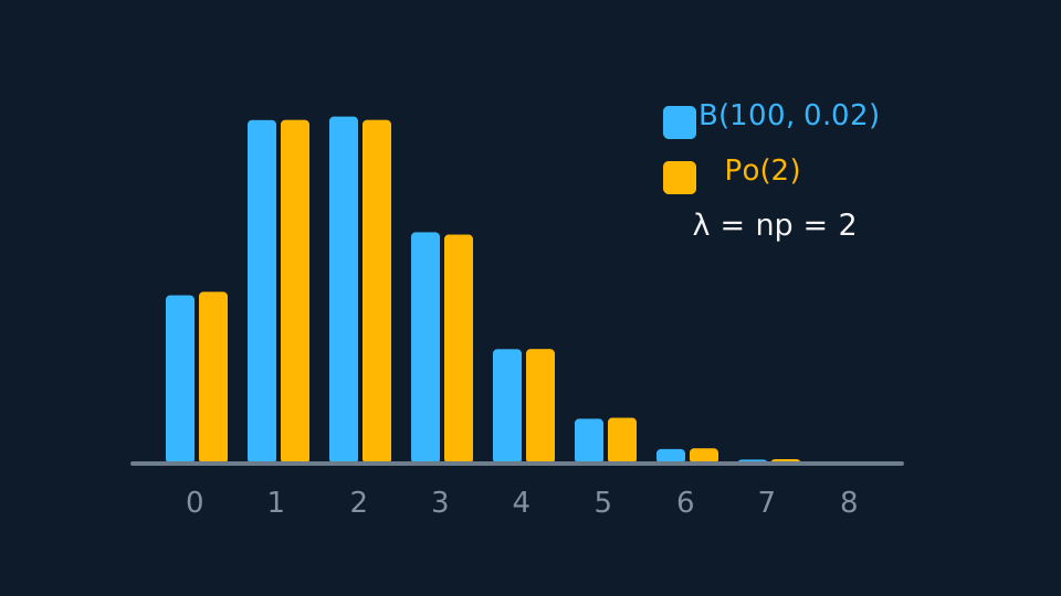
When n is large and p is small, B(n, p) is awkward to compute and close to a Poisson distribution in shape. Taking λ = np gives an approximation that improves as p shrinks, because the binomial variance np(1 − p) closes on np exactly when 1 − p is close to 1.
WORKED EXAMPLE
Rare events in many trials
A machine produces items with a 2% fault rate, independently. For a batch of 100, approximate the probability of no faults, and compare with the exact binomial value.
λ = np = 2, so P(X = 0) ≈ e⁻² = 0.135.
Exactly, 0.98¹⁰⁰ = 0.133. The two differ by less than 0.003, and the gap narrows further for smaller p.
GUIDED PRACTICE
Pooling two rates
Emails arrive at Po(4) per hour and texts at Po(1.5) per hour, independently. Find the distribution of the total number of messages in a two-hour period, and its variance.
Show the working
Per hour the total is Po(4 + 1.5) = Po(5.5) by the additive property.
Over two hours the window doubles, giving Po(11).
The variance equals the mean, so it is 11. Both the pooling and the stretching happen on λ alone.
ASSESSMENT FOCUS
- Write the distribution as X ~ Po(λ) with λ evaluated for the window in the question.
- Scale λ to the interval asked about before computing anything. Per-minute rates rarely match per-question windows.
- A Poisson distribution has its mean equal to its variance. Quote both values whenever suitability is raised.
- Name a specific condition when asked whether the model fits, such as 'events occur at a constant average rate', and say how the context may violate it.
- For the binomial approximation, say that n is large and p is small, then set λ = np.
- The additive property needs independence. Say so before you pool two counts.
CHECK YOURSELF
Accidents at a junction follow Po(2) per week. Find the mean and variance of the number of accidents in a four-week month.
Show a hint
Scale λ with the window.
Show the answer
Over four weeks the count is Po(8), so both the mean and the variance are 8.
Poisson counts events occurring singly, independently and at a constant average rate, with E(X) = Var(X) = λ.
Independent Poissons add and windows scale λ, and B(n, p) becomes Po(np) for large n and small p.
WORKBOOK
Printable practice for this topic: original exam-style questions with room to work, and a fully worked answer book. Free to use; please do not redistribute or sell.
Or read them with their worked answers on the Poisson distribution questions page.
USED LATER IN
CHECK YOUR PROGRESS
Rate how confident you feel with each objective for this lesson. Ratings are saved in this browser, on this device, unless you sign in.
- Model random events with Po(λ) and compute probabilities on a calculator.
- State the conditions a Poisson model requires and check them against a context.
- Use E(X) = Var(X) = λ, scale λ with the length of the window, and add independent counts.
- Approximate B(n, p) by Po(np) when n is large and p is small.
Open the full revision checklist to see every objective in the course in one place.