Maths › Further Statistics 2 › Least squares regression and residuals
Least squares regression and residuals
The least squares regression line minimises the sum of the squared vertical residuals. Calculate its coefficients from summary statistics, recover the line in the original variables after coding, and use the residuals and the residual sum of squares to assess whether a straight line is a suitable model.
Builds on Correlation and regression and Representing and interpreting data.
IN THIS TOPIC
- Calculate regression coefficients from summary statistics and write the line down.
- Recover the line in the original variables from one fitted to coded data.
- Compute residuals and use them to judge a fit and spot outliers.
- Find the residual sum of squares and say what it measures.
COMMON MISCONCEPTION
The least squares line is the one that passes closest to all the points, measuring distance perpendicular to the line.
The distances minimised are vertical. A residual is the gap between the observed y and the value the line predicts, y − (a + bx), and least squares makes the sum of the squares of those residuals as small as it can, which gives b = Sxy/Sxx and a line through the mean point. Minimising perpendicular distances would give a different line altogether.
Minimising the vertical gaps
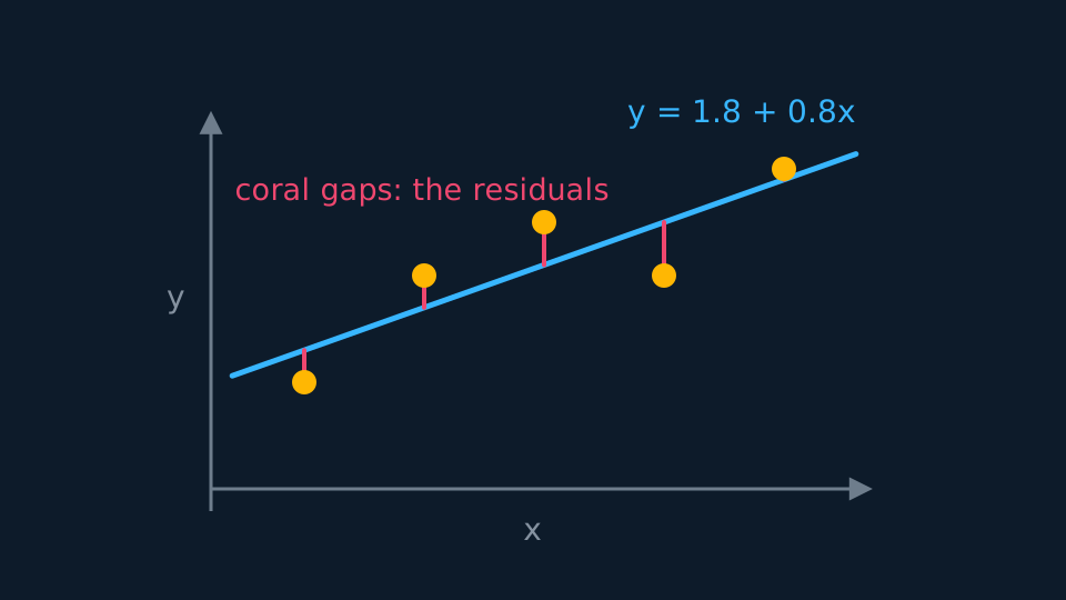
For each data point the residual is the vertical gap between the observed y and the value the line predicts, so it is y − (a + bx). The least squares line makes the sum of the squares of those residuals as small as possible. The distances measured are vertical, never perpendicular; minimising perpendicular distances would give a different line altogether.
That choice is what separates the regression of y on x from the regression of x on y. Each minimises gaps in its own direction, so the two lines differ unless the points lie exactly on one. Use y on x when x is the controlled or explanatory variable and y is the one you want to predict. Squaring keeps the algebra differentiable, and it punishes one large miss more heavily than several small ones.
Pearson Edexcel 9FM0 formulae booklet: included, under Correlation and regression, together with the computational forms of Sxx and Sxy. The second formula makes the line pass through the mean point for any data set. That gives a check on a computed line and a way to recover the intercept from the gradient and the two means.
WORKED EXAMPLE
A line from summary statistics
For the five points (1, 2), (2, 4), (3, 5), (4, 4), (5, 6), find the regression line of y on x.
Σx = 15, Σy = 21, Σx² = 55, Σxy = 71, so Sxx = 55 − 15²/5 = 10 and Sxy = 71 − (15)(21)/5 = 8.
b = 8/10 = 0.8, and a = 4.2 − 0.8 × 3 = 1.8.
The line is y = 1.8 + 0.8x. Predicted values are 2.6, 3.4, 4.2, 5.0, 5.8, and the mean point (3, 4.2) sits on the line as it must.
Fitting to coded data
Large or awkward numbers are usually coded before the summary statistics are formed, with p = (x − h)/c and q = (y − k)/d for constants of your choosing. Fit the line to the coded pairs in the ordinary way, q = A + Bp, and then undo the coding. Rearranging the two rules gives q in terms of y and p in terms of x, and substituting turns the coded line back into a line in x and y.
The gradient becomes b = dB/c and the intercept a = k + dA − dBh/c. Reading those two off: the gradient carries the scale factors alone, multiplied by the one on y and divided by the one on x, and the shifts h and k move the intercept without touching the gradient.
Compare the coefficient r, whose size the coding leaves unchanged. The difference is that r is built from a ratio in which the units cancel, while a gradient carries units of y per unit of x, so a rescaled axis has to change it. The intercept can be recovered from the mean point instead of from the formula, because the uncoded means follow from the coded ones.
WORKED EXAMPLE
Recovering a line from a coded fit
The same five points are coded as p = x − 3 and q = (y − 4)/2, giving p values −2, −1, 0, 1, 2 and q values −1, 0, 0.5, 0, 1. Fit the coded line and recover the line in x and y.
Coded summaries: mean p = 0, mean q = 0.1, Spp = 10 and Spq = 4 − 5 × 0 × 0.1 = 4.
So B = 4/10 = 0.4 and A = 0.1 − 0.4 × 0 = 0.1, and the coded line is q = 0.1 + 0.4p.
Here c = 1, d = 2, h = 3 and k = 4, so b = 2 × 0.4/1 = 0.8 and a = 4 + 2 × 0.1 − 2 × 0.4 × 3/1 = 1.8.
The line is y = 1.8 + 0.8x, which is the one fitted from the raw data above. Substituting is the same work done differently: y = 4 + 2q = 4 + 2(0.1 + 0.4(x − 3)), which tidies to the same line.
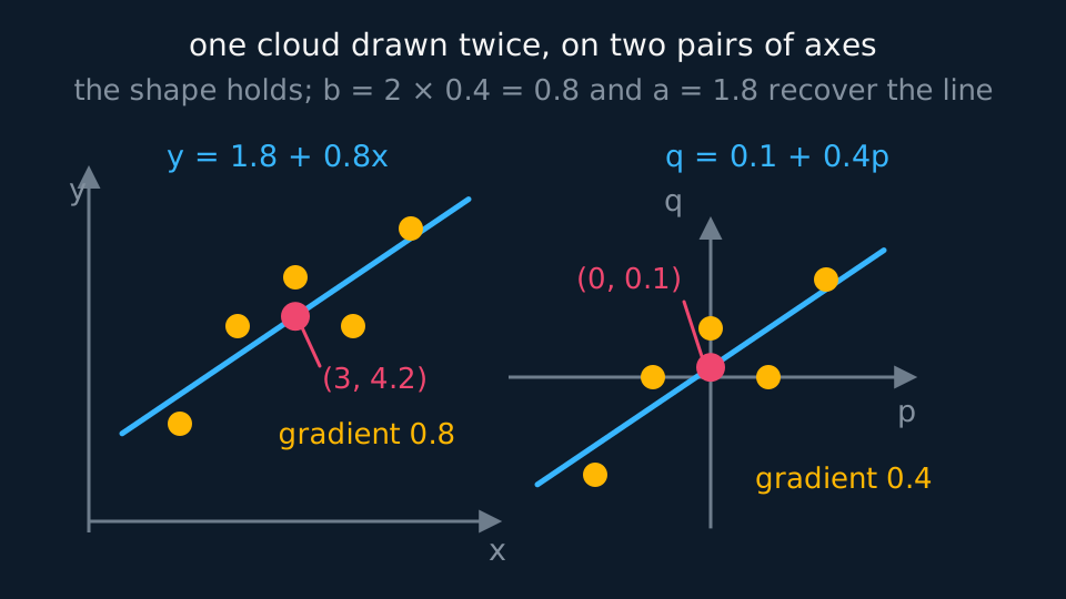
Plotted on axes scaled to match the coding, the coded points have the same arrangement as the raw points, translated but not reshaped, with the same line through them. Only the scale of the reading changes: one unit of q is two units of y, so the coded gradient is 0.4 where the raw fit gave 0.8, and b = dB/c converts between them.
Describe the drawing
Two scatter graphs side by side. On the left the five points rise about the line y = 1.8 + 0.8x, with the coral mean point at three comma four point two sitting on it. On the right the same five points are drawn against the coded axes p and q, where they make an identical shape shifted across the page, and the coral mean point has become nought comma nought point one on the line q = 0.1 + 0.4p. Only the scales on the axes have changed, which is why one gradient reads 0.8 and the other 0.4.
GUIDED PRACTICE
Undoing a coding
Values of x near 500 and y near 20 are coded as p = x − 500 and q = 5(y − 20). The fitted coded line is q = 3 + 2p. Find the regression line of y on x.
Show the working
Reading the coding as q = (y − k)/d needs d = 1/5 and k = 20, while c = 1 and h = 500.
Gradient: b = dB/c = (1/5) × 2 = 0.4.
Intercept: a = k + dA − dBh/c = 20 + 0.6 − 0.4 × 500 = −179.4, so the line is y = −179.4 + 0.4x.
Check it at x = 500: y = 20.6, and the coded line at p = 0 gives q = 3, that is y = 20 + 3/5 = 20.6. Substituting q = 5(y − 20) and p = x − 500 into q = 3 + 2p gives the line in one step and is worth doing when the constants are hard to see.
Interpreting residuals
Plot the residuals against x. If a straight line is the right model they scatter about zero with no pattern. A curve in the residual plot means the relationship was not linear and a transformation is needed. A fan shape means the spread of y grows with x, which breaks the assumption behind the fit even though the line itself may look fine.
One residual far larger than the rest indicates a possible outlier or a recording error. Investigate it before deleting it, and state in your answer why you would or would not drop the point.
For an ordinary least-squares regression that includes an intercept, the residuals sum to zero, apart from rounding, so their sizes carry the information and their total carries none. The property follows from fitting the intercept: choosing a to minimise the sum of squares is the condition Σ(y − a − bx) = 0. It need not hold for a regression constrained through a fixed point.
The residual sum of squares
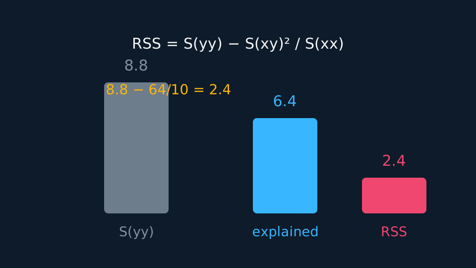
Add the squares of the residuals and you have a single number for what the line failed to explain:
Pearson Edexcel 9FM0 formulae booklet: included, with the equivalent Syy(1 − r²) beside it, which is the shorter route when r is already known. Syy is the total variation in y, so the subtracted term is the part the line accounts for. A small RSS relative to Syy means the line has done most of the work. Squaring the residuals directly gives the same answer, and comparing the two routes is a good way to check a slip.
GUIDED PRACTICE
Residuals and RSS
For the same five points, find the residuals and the residual sum of squares, and comment.
Show the working
Observed minus predicted: −0.6, 0.6, 0.8, −1.0, 0.2. They sum to zero, as they must for a fitted line with an intercept.
Sum of squares: 0.36 + 0.36 + 0.64 + 1.00 + 0.04 = 2.4.
By the formula: Syy = 97 − 21²/5 = 8.8, so RSS = 8.8 − 64/10 = 2.4, which agrees.
The line explains 6.4 of the 8.8 total variation. The largest residual, −1.0 at x = 4, is not extreme enough to call an outlier.
ASSESSMENT FOCUS
- Quote the formulae for the coefficients and show the summary statistics you put into them.
- After fitting to coded data, say which line you have. A line in p and q answers nothing until it is turned back into x and y.
- Undo a coding by substituting the two coding rules into the fitted line rather than by recalling a formula for the intercept.
- Residual means observed minus predicted; the reverse order changes the sign of every residual.
- Interpret a residual plot in words. A systematic pattern is evidence against the linear model; scatter with no pattern is consistent with it.
- For the RSS, either sum the squared residuals or use the formula, and say which route you took.
CHECK YOURSELF
A regression line gives Sxx = 20, Sxy = 30 and Syy = 50. Find the gradient and the residual sum of squares.
Show a hint
One division for the gradient, then the RSS formula.
Show the answer
b = 30/20 = 1.5. RSS = 50 − 900/20 = 50 − 45 = 5, so the line explains 45 of the 50 total variation.
Least squares minimises the sum of the squared vertical residuals, giving b = S(xy)/S(xx), with the line through the mean point.
Coding by p = (x − h)/c and q = (y − k)/d scales the gradient by d/c and leaves the shifts to the intercept, so substitute the coding rules back to recover the line.
For a least-squares fit with an intercept the residuals sum to zero, their pattern tests the model, and RSS = S(yy) − S(xy)²/S(xx) measures what is left unexplained.
WORKBOOK
Printable practice for this topic: original exam-style questions with room to work, and a fully worked answer book. Free to use; please do not redistribute or sell.
Or read them with their worked answers on the least squares regression and residuals questions page.
CHECK YOUR PROGRESS
Rate how confident you feel with each objective for this lesson. Ratings are saved in this browser, on this device, unless you sign in.
- Calculate regression coefficients from summary statistics and write the line down.
- Recover the line in the original variables from one fitted to coded data.
- Compute residuals and use them to judge a fit and spot outliers.
- Find the residual sum of squares and say what it measures.
Open the full revision checklist to see every objective in the course in one place.