Maths › Statistics › Correlation and regression
Correlation and regression
Use scatter diagrams and the product moment correlation coefficient to describe the direction and strength of linear association. Use a least-squares regression line to predict the response variable within the observed range, and distinguish association from causation.
Builds on Representing and interpreting data and Straight lines.
IN THIS TOPIC
- Describe correlation from a scatter diagram and interpret a product moment correlation coefficient r between −1 and 1.
- Use a regression line y = a + bx to make predictions, interpreting a and b in context.
- State the limitations of a prediction, and identify a possible confounding variable where correlation is being treated as evidence of cause.
- Take logs to straighten y = axn and y = kbx, then read the constants off the regression line.
COMMON MISCONCEPTION
A correlation of r = 0.9 proves that changing one variable causes the other to change.
r measures the direction and strength of a linear association, and an association is not a mechanism. A third variable can move both: ice cream sales and drowning rates both rise in warmer weather. A causal conclusion needs a study design and evidence that address plausible confounding, whatever the value of r.
Reading a scatter graph
Describe the drawing
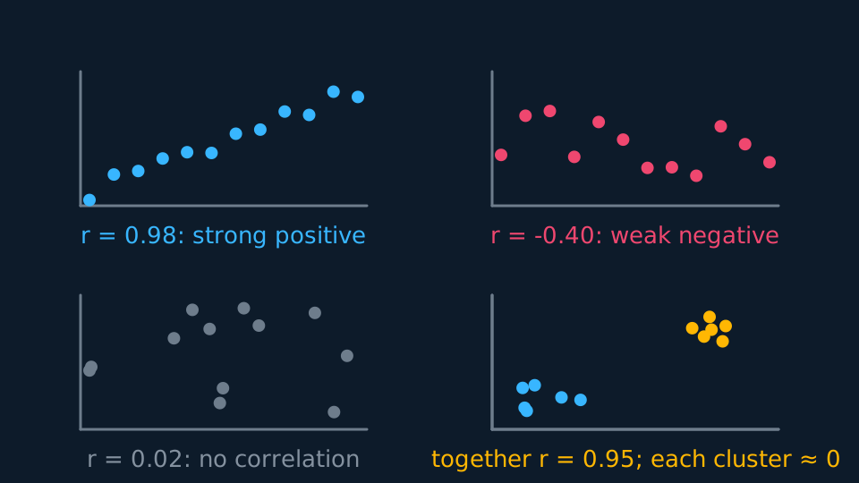
Four small scatter panels, each captioned with the correlation computed from its own points: a tight rising cloud with r near one, a loose falling cloud with r about minus a third, a shapeless cloud with r near zero, and a fourth panel of two separate clusters whose twelve points together give a large r although neither cluster alone shows any correlation.
Plot one variable against another. Points rising together show positive correlation; one variable falling as the other rises shows negative correlation; a scatter with no linear trend shows no linear correlation. The product moment correlation coefficient r measures linear association and always lies between −1 and 1. The sign gives the direction and the magnitude the strength; r = ±1 means the points lie exactly on a straight line.
A calculator computes r from the data; the interpretation must be stated in context, giving strength, direction and the variables. For example: “r = 0.96 shows strong positive linear correlation, so taller plants tend to carry more fruit.”
Examine the scatter diagram as well as r. A diagram may show two separate clusters, for example by sex or by season, and a single r calculated across both describes neither group; state this where it occurs.
The regression line
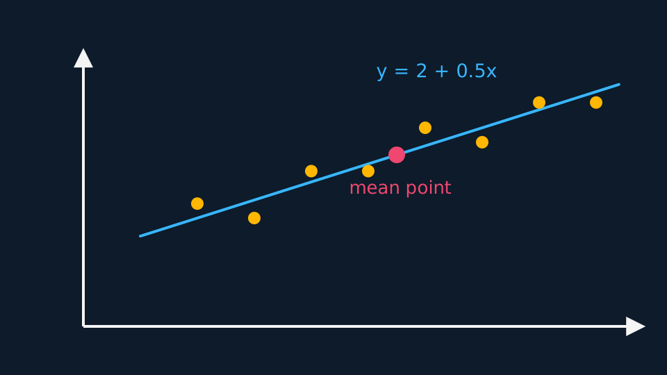
The least squares regression line y = a + bx is the straight line minimising the sum of the squared vertical distances from the points. For ordinary least squares with an intercept term, that line passes through the mean point of the data and the residuals sum to zero. Interpret a and b in context: b is the change in y associated with each extra unit of x, and a is the predicted y when x is zero, which may or may not correspond to a possible situation.
WORKED EXAMPLE
Interpreting a and b
For ice cream sales s (pounds) against temperature t (°C), a calculator gives s = 42 + 15.3t. Interpret the numbers.
The gradient: each extra degree is associated with about £15.30 more in daily sales.
The intercept: £42 of sales predicted at 0 °C. Plausible as a baseline, though 0 °C may sit outside the temperatures collected.
State the relationship as association: write “associated with” rather than “causes”, and use the units of the problem.
Interpolation, extrapolation and causation
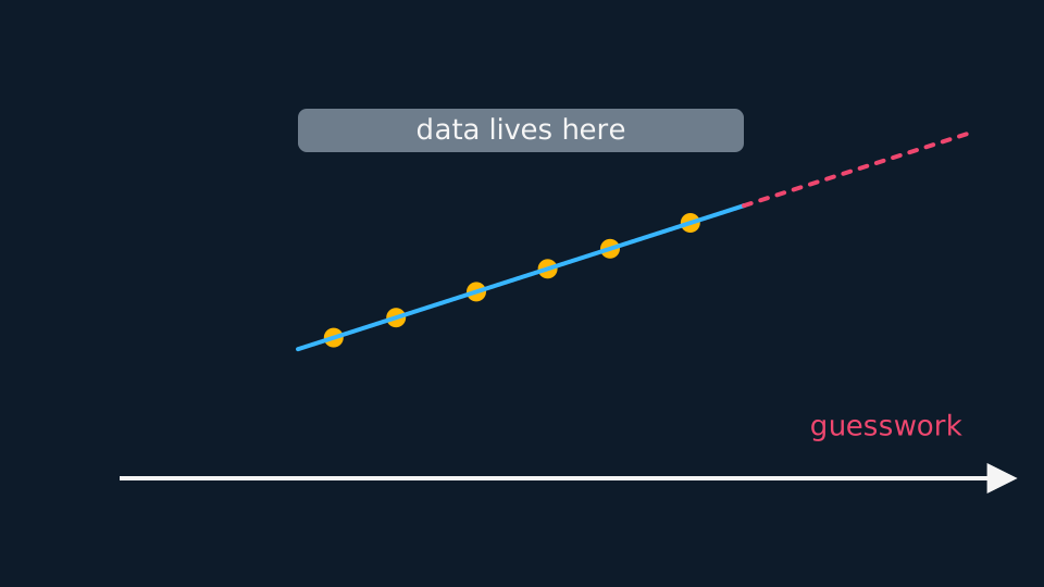
Predicting within the range of observed x values is interpolation. It avoids the additional risk of extrapolation but is still affected by scatter, model fit, measurement quality and any unrepresented groups in the data. Predicting outside the observed range is extrapolation: the line still returns a number, but no data support the model there, so state that the prediction is unreliable.
The line of y on x is fitted to predict y from x, with x the explanatory variable and y the response; using it in reverse to estimate x from y is not valid. Correlation describes linear association and does not establish causation, however large r is. A third variable may influence both measured variables: ice cream sales and drowning rates both increase in warmer weather. A causal conclusion needs an appropriate study design and evidence that address plausible confounding.
Straightening a curve with logs
Not every relationship is linear, and two curved ones straighten under logarithms. For y = axn, taking logs of both sides gives log y = log a + n log x, so plotting log y against log x should give a straight line of gradient n and intercept log a. For y = kbx, log y = log k + x log b, so log y against x is the straight one.
Fit the regression line to the transformed data, then convert back. A line log y = 0.42 + 1.6 log x gives n = 1.6 and a = 100.42 ≈ 2.63, so y ≈ 2.63x1.6. Only the intercept requires conversion by a power of ten here; the gradient is already n. State which axis was logged before converting back.
ASSESSMENT FOCUS
- Interpret r in one sentence giving strength, direction and context rather than restating the value.
- Read b as “for each extra unit of x, y changes by b” in the question's own units, and read a as the prediction at x = 0, then state whether that value is meaningful here.
- Predict only for x within the observed range, and only from the line of y on x. For any other prediction, state that it is unreliable and give the reason.
- When stating that correlation does not establish causation, name a plausible third variable in the context of the question.
- For log models, state which variable was logged, and convert the intercept back correctly when recovering the original constants.
CHECK YOURSELF
A regression line for crop yield y (tonnes) against rainfall x (cm), from data with 20 ≤ x ≤ 60, is y = 1.2 + 0.08x. A farmer asks for the predicted yield when x = 100. What do you say?
Show a hint
Where does 100 sit relative to the data?
Show the answer
The line gives 1.2 + 0.08 × 100 = 9.2 tonnes, but x = 100 is far outside the observed range 20 to 60.
That is extrapolation, so the prediction is unreliable: the linear pattern need not continue beyond x = 60.
r measures the direction and strength of a linear association, not causation.
Regress y on x, predict only inside the data, and read a and b in the question's own units.
WORKBOOK
Printable practice for this topic: original exam-style questions with room to work, and a fully worked answer book. Free to use; please do not redistribute or sell.
Or read them with their worked answers on the correlation and regression questions page.
USED LATER IN
CHECK YOUR PROGRESS
Rate how confident you feel with each objective for this lesson. Ratings are saved in this browser, on this device, unless you sign in.
- Describe correlation from a scatter diagram and interpret a product moment correlation coefficient r between −1 and 1.
- Use a regression line y = a + bx to make predictions, interpreting a and b in context.
- State the limitations of a prediction, and identify a possible confounding variable where correlation is being treated as evidence of cause.
- Take logs to straighten y = axn and y = kbx, then read the constants off the regression line.
Open the full revision checklist to see every objective in the course in one place.