Maths › Further Statistics 2 › Continuous random variables: density and distribution functions
Continuous random variables: density and distribution functions
A continuous random variable can take any value in a range, so probabilities attach to intervals rather than to single values. The probability density function gives those probabilities as areas and the cumulative distribution function accumulates them. Use F to find percentiles and the distribution of a function of X, handle variables that are part discrete and part continuous, and, where the specification includes it, use the exponential distribution as the wait between Poisson events.
Builds on The normal distribution and Definite integrals and areas and The Poisson distribution.
IN THIS TOPIC
- Check that a proposed density is valid and use it to find probabilities.
- Move between the density and the cumulative distribution function in both directions.
- Use the distribution function to find the median and other percentiles.
- Find the distribution of a function of X by rewriting its event and differentiating back.
- Work with a variable that is part discrete and part continuous.
- Write down the exponential distribution as the wait between Poisson events and use it.
- Prove the memoryless property from the exponential tail, and say which situations it suits and which it does not.
COMMON MISCONCEPTION
For a continuous random variable, P(X = 1.5) is the height of the density at 1.5.
The area over a single point is zero, so P(X = c) = 0 for every c and the height f(c) is not a probability at all. Probability is area under the density: the chance that X falls between a and b is the integral of f from a to b. A density may even exceed 1 on a short interval and stay valid, since only the total area is constrained.
Probability as area under the density
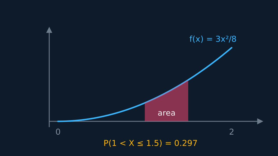
A probability density function f(x) is never a probability. It is non-negative, its total area is 1, and probabilities are the areas beneath it:
Pearson Edexcel 9FM0 formulae booklet: the cumulative version F(x₀) = P(X ≤ x₀), as the integral of f from the bottom of the range up to x₀, is included; this two-limit form is not. The area over a single point is zero, so P(X = c) = 0 for every c: the height f(c) is not a probability. A density may exceed 1 on a short interval without being invalid, since only the total area is constrained. Because P(X = c) = 0, strict and non-strict inequalities give the same probability for a continuous variable, unlike a discrete one.
WORKED EXAMPLE
Checking a density and using it
f(x) = 3x²/8 for 0 ≤ x ≤ 2 and zero elsewhere. Verify it is a density and find P(1 < X ≤ 1.5).
It is non-negative on the interval. Its integral is [x³/8] from 0 to 2 = 8/8 = 1, so it is valid.
P(1 < X ≤ 1.5) = [x³/8] from 1 to 1.5 = 3.375/8 − 1/8 = 0.297 to three decimal places.
The distribution function
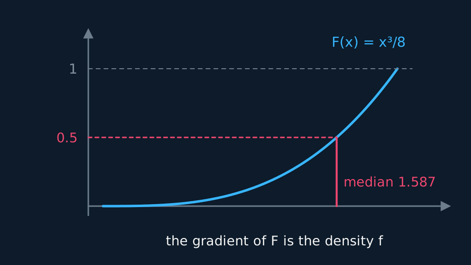
The cumulative distribution function collects everything to the left, so F(x0) = P(X ≤ x0), the integral of f from the lower end up to x0. It climbs from 0 to 1 and never falls. Differentiating undoes the integration:
Pearson Edexcel 9FM0 formulae booklet: F is defined there as an integral of f, but this reverse relation is not stated. F is the more direct route to a probability, since P(a < X ≤ b) is just F(b) − F(a). f is the better tool for describing shape. Percentiles come from F, with the median m solving F(m) = 0.5 and the lower quartile solving F(q) = 0.25. Piecewise definitions need every branch stated, including the 0 below the range and the 1 above it.
GUIDED PRACTICE
From density to median
For f(x) = 3x²/8 on 0 ≤ x ≤ 2, write down F(x) in full and find the median.
Show the working
Integrating from 0: F(x) = x³/8 on the interval. In full, F(x) = 0 for x < 0, x³/8 for 0 ≤ x ≤ 2, and 1 for x > 2.
The median solves m³/8 = 0.5, so m³ = 4 and m = 1.587 to three decimal places.
Checking: F(1.587) = 3.997/8 ≈ 0.5, and the value sits inside the range as it must.
The distribution of a function of X
Given the distribution of X, the distribution of a function of it, such as Y = X³ or a length converted into another unit, is found from F rather than from f. Write FY(y) = P(Y ≤ y), rewrite the event Y ≤ y as a statement about X alone, and evaluate its probability with FX. Differentiating that expression returns the density of Y, and the range of Y is the range of X put through the same rule.
Two errors to avoid. Rearranging by a decreasing rule turns the inequality round, so P(Y ≤ y) becomes P(X ≥ something), and that is 1 − FX of it rather than FX. The other is substituting into the density instead: fX(y1/3) is not the density of Y, because differentiating FY sends the chain rule through the substitution and picks up a factor that the swap leaves out. Going by way of F carries that factor for you.
WORKED EXAMPLE
The cube of a continuous variable
X has density f(x) = 3x²/8 on 0 ≤ x ≤ 2, so F(x) = x³/8 there. Find the distribution function and the density of Y = X³.
X runs from 0 to 2, so Y = X³ runs from 0 to 8.
Cubing is increasing, so X³ ≤ y says the same thing as X ≤ y1/3. Then for 0 ≤ y ≤ 8, FY(y) = P(X ≤ y1/3) = (y1/3)³/8 = y/8, with 0 below and 1 above.
Differentiating, fY(y) = 1/8 for 0 ≤ y ≤ 8: the cube of this X is uniform on that interval.
Two checks. A constant 1/8 across a width of 8 has area 1, so it is a valid density. And E(Y) is E(X³) = ∫ x³ × 3x²/8 dx from 0 to 2 = 4, which is the midpoint of 0 to 8, where a uniform mean belongs.
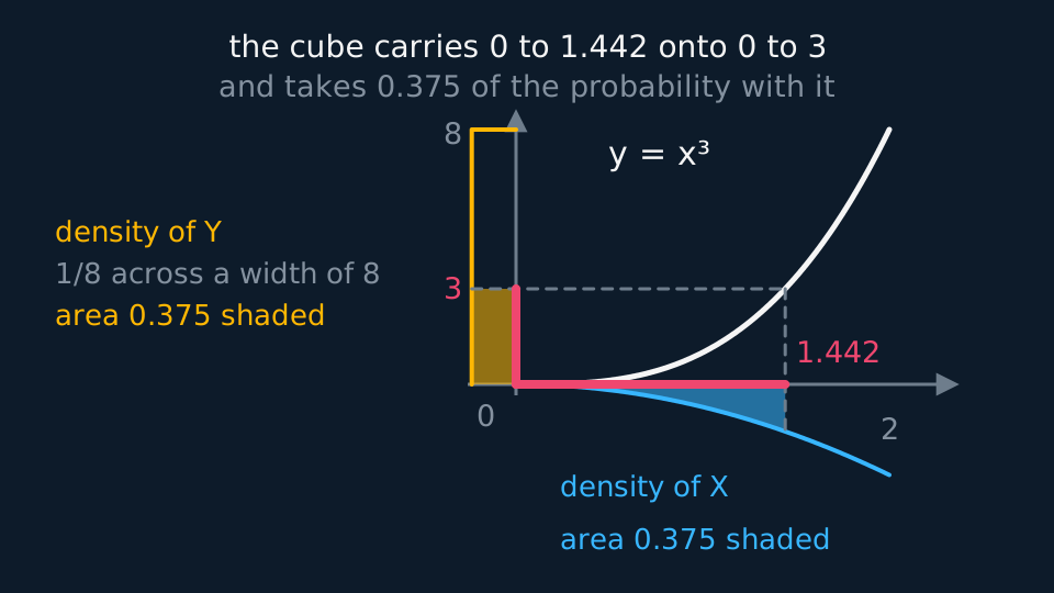
Cubing carries the interval from 0 to 1.442 on the x-axis onto the interval from 0 to 3 on the y-axis, and the probability is preserved: the area under fX over the first equals the area under fY over the second, and both are 0.375.
Describe the drawing
The curve y = x cubed climbing from the origin, with the interval from nought to one point four four two marked on the horizontal axis and the interval from nought to three marked on the vertical. Below the horizontal axis hangs the density of X, three x squared over eight, shaded over the first interval; to the left of the vertical axis stands the density of Y, flat at an eighth across a width of eight, shaded over the second. The two shaded patches have the same area, nought point three seven five, because they are the same probability read on either variable.
GUIDED PRACTICE
A rule that runs backwards
For the same X, with F(x) = x³/8 on 0 ≤ x ≤ 2, find the density of Y = 2 − X and the median of Y.
Show the working
Y runs from 0 to 2. Subtracting turns the inequality round: FY(y) = P(2 − X ≤ y) = P(X ≥ 2 − y) = 1 − (2 − y)³/8 on 0 ≤ y ≤ 2.
Differentiating gives fY(y) = 3(2 − y)²/8 on 0 ≤ y ≤ 2. Its integral across the range is 1, as a density's has to be.
The median solves 1 − (2 − m)³/8 = 0.5, so (2 − m)³ = 4 and m = 2 − 1.587 = 0.413. That is the median of X reflected in 1, which is what subtracting from 2 does to a value.
Mixed discrete and continuous distributions
Some variables are part discrete and part continuous. A wait at a counter is zero whenever a server is free, an outcome with a probability of its own, and takes positive values otherwise. Such a variable carries a positive probability at a single value alongside a density elsewhere, and the two parts share one total:
The sum runs over the values carrying positive probability, often just one, and the integral over the range on which the density is defined. Setting the total to 1 determines an unknown constant in either part. The distribution function again collects everything to the left, so it increases where the density is positive and has a jump at each value carrying positive probability. The size of the jump is that probability: P(X = c) is F(c) minus the limit of F from below. Elsewhere the continuous reading stands, and a single value carries no probability.
Expectations split in the same way. E(X) weights each discrete value by its probability and adds the integral of xf(x) over the continuous part, and E(X²) is assembled from the same two pieces, so the variance follows as before.
WORKED EXAMPLE
A wait that is often zero
A driver reaches a set of lights. The light is green on arrival with probability 0.4, so the wait T is 0 seconds; otherwise the wait is spread evenly, with f(t) = 0.02 for 0 < t ≤ 30. Find P(T ≤ 10), the median and the mean wait.
First the total: 0.4 + 0.02 × 30 = 0.4 + 0.6 = 1, so the model is valid.
F(t) = 0.4 + 0.02t on 0 ≤ t ≤ 30, stepping from 0 to 0.4 at t = 0 and reaching 1 at t = 30. So P(T ≤ 10) = 0.4 + 0.2 = 0.6.
The median solves 0.4 + 0.02m = 0.5, giving m = 5 seconds, which lies in the continuous part rather than at t = 0.
E(T) = 0 × 0.4 + ∫ 0.02t dt from 0 to 30 = 0.02 × 450 = 9 seconds.
The exponential distribution
Board scope. The exponential distribution is included in AQA 7367 optional statistics and OCR H245 statistics. It is not listed in Pearson Edexcel 9FM0 Further Statistics. The density is f(x) = λe−λx and the distribution function is F(x) = 1 − e−λx, for x ≥ 0.
Take events landing at random at a constant mean rate λ, singly and independently, which are the conditions behind a Poisson model. Fix any moment and let X be the wait until the next event. X is continuous and non-negative, and its distribution takes one line to find, because X is longer than x when no event lands in the next x units of time. Counts over a window of length x follow Po(λx), and the probability of a count of zero is e−λx. That is the tail of X, and taking it from 1 leaves the distribution function of the exponential distribution:
Differentiating F returns the density, which is the function the distribution is named after:
Below zero both functions are 0, and for positive x F climbs towards 1 without reaching it, so the wait has no upper limit. λ is a rate, counted in events per unit of time or of distance, and x is measured in that same unit, so a mean wait of m goes with λ = 1/m.
Probabilities come from either function, as they do for any continuous variable. With F written down, an interval is a subtraction, so P(a < X < b) is e−λa − e−λb, and a tail needs no subtraction at all. Integrating the density gives the same numbers, because the integral of λe−λt across an interval is −e−λt evaluated at its ends. Before substituting, read the rate, identify the unit it is counted in, and convert the window into that unit.
Converting the variable itself is the same conversion done once, by the transformation method above. With X the wait in hours and Y = 60X the same wait in minutes, P(Y ≤ y) = P(X ≤ y/60) = 1 − e−λy/60, which is the exponential distribution function again with rate λ/60. So emails at 4 an hour are emails at 1/15 a minute, and a mean wait of a quarter of an hour reads as 15 minutes. Scaling an exponential wait leaves it exponential and divides the rate by the scale factor.
WORKED EXAMPLE
Three probabilities from one rate
Emails arrive at random at a mean rate of 4 per hour. Find the probability that the wait for the next one is under 15 minutes, the probability it is over 30 minutes, and the probability it falls between 10 and 30 minutes.
Working in hours, λ = 4, and the three windows are 0.25, 0.5 and 1/6 to 0.5.
P(X < 0.25) = 1 − e⁻¹ = 0.632.
P(X > 0.5) = e⁻² = 0.135.
P(1/6 < X < 0.5) = e−2/3 − e⁻² = 0.513 − 0.135 = 0.378. Integrating 4e−4t between the same limits returns the same figure, which is a check worth making once.
The memoryless property
The memoryless property follows from the tail. Suppose the wait has already run for s with no event. The probability of a further t is a conditional probability, and the two tails divide: e−λ(s + t) over e−λs leaves e−λt, the probability of a wait of t measured from the start.
The time already spent waiting therefore does not affect the distribution of the remaining wait, which restates the modelling conditions: events occur at a constant rate, independently of when the last one occurred. The model suits arrivals, calls and radioactive decay, and is unsuitable where components wear: a bearing that has turned for a year may be more likely to fail this month than a new one, and an exponential model cannot represent that.
GUIDED PRACTICE
The memoryless property
The lifetime of a bulb is modelled by an exponential distribution with a mean of 2000 hours. Find the probability that a new bulb lasts beyond 3000 hours, and the probability that a bulb already burning at 1000 hours lasts beyond 4000.
Show the working
The mean is 1/λ, so λ = 1/2000 per hour, and P(X > 3000) = e−1.5 = 0.223.
For the second, the further wait beyond 1000 hours has the same distribution as a fresh one, so the answer is P(X > 3000) = 0.223 again. The long way agrees: e⁻² divided by e−0.5 is e−1.5.
A bulb that survives to any age faces the distribution of remaining life it faced when new. Where components wear, that assumption fails and the model is the wrong one.
ASSESSMENT FOCUS
- Verify a density by checking both conditions, non-negative and total area exactly 1.
- Write a piecewise F(x) with every branch, including the flat 0 and the flat 1.
- Read probabilities from F by subtraction: P(a < X ≤ b) = F(b) − F(a), rather than re-integrating the density.
- For a percentile, set F equal to the proportion and solve, then check the root lies in range.
- When f is defined in pieces, build F piece by piece and make the branches agree where they meet.
- For a function of X, start at P(Y ≤ y), rearrange into an event about X, and turn the inequality round if the rule is decreasing.
- Give the range of Y with its density, taking the ends of the range of X through the same rule.
- For a part discrete, part continuous variable, add the lumps to the area and set the total to 1 before anything else.
- For an exponential model, say which unit the rate is counted in and convert the window to match before substituting.
- λ is a rate, so a mean wait of m gives λ = 1/m. Substituting the mean for λ inverts the parameter and gives the wrong probability.
CHECK YOURSELF
f(x) = kx for 0 ≤ x ≤ 4 and zero elsewhere. Find k and F(x) on the interval.
Show a hint
Total area 1 fixes k, then integrate from the lower end.
Show the answer
The area is k[x²/2] from 0 to 4 = 8k, so k = 1/8. Then F(x) = x²/16 on 0 ≤ x ≤ 4, with F = 0 below and F = 1 above.
For a continuous variable, probability is area under the density: P(a < X ≤ b) is the integral of f from a to b, and P(X = c) = 0.
F is the integral of f from the lower end, climbing from 0 to 1; differentiating F gives f back, F(m) = 0.5 gives the median, and the distribution of a function of X comes from rewriting its event in terms of X.
A part discrete, part continuous variable carries positive probability at individual values: those probabilities and the area under the density total 1, and F jumps at each such value by that probability.
Where the specification includes it, the wait between events at a constant random rate λ is exponential, with F(x) = 1 − e−λx and tail e−λx for x ≥ 0, and the memoryless property gives P(X > s + t | X > s) = P(X > t).
WORKBOOK
Printable practice for this topic: original exam-style questions with room to work, and a fully worked answer book. Free to use; please do not redistribute or sell.
Or read them with their worked answers on the continuous random variables: density and distribution functions questions page.
USED LATER IN
CHECK YOUR PROGRESS
Rate how confident you feel with each objective for this lesson. Ratings are saved in this browser, on this device, unless you sign in.
- Check that a proposed density is valid and use it to find probabilities.
- Move between the density and the cumulative distribution function in both directions.
- Use the distribution function to find the median and other percentiles.
- Find the distribution of a function of X by rewriting its event and differentiating back.
- Work with a variable that is part discrete and part continuous.
- Write down the exponential distribution as the wait between Poisson events and use it.
- Prove the memoryless property from the exponential tail, and say which situations it suits and which it does not.
Open the full revision checklist to see every objective in the course in one place.