Maths › Further Statistics 2 › Mean, variance and skewness of continuous variables
Mean, variance and skewness of continuous variables
For continuous random variables, the mean and variance follow the discrete formulae with the sums replaced by integrals. Locate the mode, median and percentiles, describe skew from the order of the mean, median and mode, and prove the mean and variance of an exponential wait.
Builds on Density and distribution functions and Discrete random variables and expectation.
IN THIS TOPIC
- Find the mean, variance and E(g(X)) for a continuous variable by integration.
- Locate the mode, median and percentiles and distinguish them.
- Describe skewness from the ordering of the three averages and justify it.
- Apply the coding results E(aX + b) and Var(aX + b) in the continuous case.
- Prove that an exponential wait has mean 1/λ and variance 1/λ², and read off its median.
COMMON MISCONCEPTION
The mode of a continuous distribution is the value that occurs most often.
No individual value occurs at all for a continuous variable, so that discrete definition does not fit. The mode is the value at which the density is greatest: differentiate f and solve f'(x) = 0, then check the ends of the range as well, because a density that falls throughout its range peaks at its left-hand endpoint and the calculus will not find it.
Sums become integrals
Every discrete formula carries over with Σ replaced by ∫ and P(X = x) replaced by f(x) dx:
Pearson Edexcel 9FM0 formulae booklet: included, under Continuous distributions, with the variance written as ∫x²f(x) dx − μ² and with E(g(X)) = ∫g(x)f(x) dx. That last result gives E(g(X)) directly, so the distribution of g(X) is not needed first. Limits are the ends of the range where f is non-zero. The coding results survive untouched, so E(aX + b) = aE(X) + b and Var(aX + b) = a²Var(X) exactly as before.
WORKED EXAMPLE
Mean and variance by integration
For f(x) = 3x²/8 on 0 ≤ x ≤ 2, find the mean and variance.
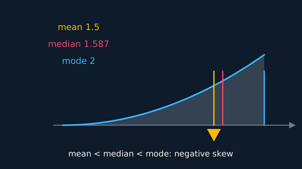
E(X) = ∫ 3x³/8 dx = [3x⁴/32] from 0 to 2 = 48/32 = 1.5.
E(X²) = ∫ 3x⁴/8 dx = [3x⁵/40] from 0 to 2 = 96/40 = 2.4.
Var(X) = 2.4 − 1.5² = 0.15, so the standard deviation is about 0.387.
Mode, median and the percentiles between them
The mode is the value where the density is greatest. Differentiate f and solve f'(x) = 0, but check the ends of the range as well, because a density that falls throughout its range peaks at its left-hand endpoint and the calculus will not find it. A mode is not a value that occurs often, since no individual value occurs at all; that definition belongs to discrete variables.
The median solves F(m) = 0.5. Any percentile works the same way, with the pth percentile solving F(x) = p/100, so the quartiles come from 0.25 and 0.75. When F is piecewise, check which branch the answer belongs in before you solve, and reject a root that lands outside the range.
WORKED EXAMPLE
A percentile from a piecewise F
F(x) = x²/16 on 0 ≤ x ≤ 4, with the usual flat branches. Find the interquartile range.
Lower quartile: q²/16 = 0.25 gives q² = 4, so q1 = 2.
Upper quartile: q²/16 = 0.75 gives q² = 12, so q3 = 3.46 to three significant figures.
The interquartile range is 1.46. Both roots lie in 0 to 4, and the negative roots are discarded.
Mean, median, mode and skew
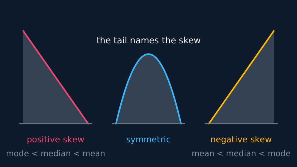
Skew describes which tail of a distribution is the longer: positive skew has the longer tail to the right, negative skew to the left. For a symmetric distribution the mean, median and mode coincide.
For a single-peaked density, mode < median < mean is an indicator of positive skew and mean < median < mode an indicator of negative skew. Treat the ordering as an indicator rather than a definition: it holds for the unimodal densities set at this level but can mislead for others, and the converse is weaker still, since three averages coinciding does not prove a density symmetric. In a justification, quote the ordering and name the tail it indicates.
GUIDED PRACTICE
Naming the skew
For f(x) = 2(1 − x) on 0 ≤ x ≤ 1, find the mean, median and mode, and describe the skew.
Show the working
E(X) = ∫ 2x(1 − x) dx = 2(1/2 − 1/3) = 1/3.
F(x) = 2x − x², so the median solves x² − 2x + 0.5 = 0, giving m = 1 − √0.5 = 0.293.
The density falls throughout the range, so the mode sits at the left-hand end, 0.
Mode 0 < median 0.293 < mean 0.333, so the distribution is positively skewed, with its tail to the right.
The mean and variance of an exponential wait
The exponential density λe−λx on x ≥ 0, the wait between Poisson events, gives integrals over an infinite range. Both proofs turn on one fact: as x grows, e−λx falls faster than any power of x climbs, so xe−λx and x²e−λx approach zero. Without that the integrals would not settle.
Integrate by parts, differentiating the power and integrating the exponential. E(X) is −xe−λx evaluated from 0 to infinity plus the integral of e−λx over the same range. The bracket is zero at both ends, and the integral left behind is 1/λ. The same parts on x² give a bracket of zero again and 2/λ times the first integral, so E(X²) = 2/λ². Subtracting the square of the mean leaves:
The standard deviation is therefore 1/λ, equal to the mean, for every exponential distribution. The median solves 1 − e−λm = 0.5, so it is (ln 2)/λ, about 0.69 of the mean, and the density is greatest at x = 0, so the mode is 0. Mode < median < mean here, and the density does have its longer tail to the right, so the distribution is positively skewed.
WORKED EXAMPLE
Mean, median and spread of a wait
Emails arrive at random at a mean rate of 4 per hour, so the wait is exponential with λ = 4. Find the mean wait, the standard deviation and the median wait, in minutes.
Mean 1/4 hour = 15 minutes, and the standard deviation is the same, 15 minutes.
Median (ln 2)/4 hour = 0.1733 hour = 10.4 minutes to three significant figures.
The median sits well below the mean, so a typical wait is shorter than the average one, and quoting the mean alone would overstate what most people experience.
ASSESSMENT FOCUS
- State the integral with its limits before evaluating. The limits are the ends of the range, not zero to infinity.
- Use E(X²) − [E(X)]², and keep the square of the mean intact until the last line.
- For the mode, differentiate f, then check the endpoints too. A monotonic density peaks at an end.
- Justify skew by quoting the order of the three averages as an indicator, and name which side the longer tail lies on.
- Integrating over an infinite range, say why the bracket vanishes at the top: the exponential outruns the power.
CHECK YOURSELF
For f(x) = 1/4 on 0 ≤ x ≤ 4, find E(X) and E(X²).
Show a hint
Integrate x and x² against the constant density.
Show the answer
E(X) = ∫ x/4 dx = [x²/8] from 0 to 4 = 2. E(X²) = [x³/12] from 0 to 4 = 64/12 = 16/3, so Var(X) = 16/3 − 4 = 4/3.
Replace sums with integrals: E(X) is the integral of xf(x), E(g(X)) the integral of g(x)f(x), and Var(X) = E(X²) − [E(X)]².
The mode is where f peaks, endpoints included, any percentile solves F(x) = p/100, and for a single-peaked density the order of the three averages indicates the skew.
An exponential wait has mean 1/λ, variance 1/λ² and median (ln 2)/λ, proved by parts once you know the exponential outruns the power.
WORKBOOK
Printable practice for this topic: original exam-style questions with room to work, and a fully worked answer book. Free to use; please do not redistribute or sell.
Or read them with their worked answers on the mean, variance and skewness of continuous variables questions page.
CHECK YOUR PROGRESS
Rate how confident you feel with each objective for this lesson. Ratings are saved in this browser, on this device, unless you sign in.
- Find the mean, variance and E(g(X)) for a continuous variable by integration.
- Locate the mode, median and percentiles and distinguish them.
- Describe skewness from the ordering of the three averages and justify it.
- Apply the coding results E(aX + b) and Var(aX + b) in the continuous case.
- Prove that an exponential wait has mean 1/λ and variance 1/λ², and read off its median.
Open the full revision checklist to see every objective in the course in one place.