Maths › Statistics › The binomial distribution
The binomial distribution
The binomial distribution models the number of successes in a fixed number of independent trials, each with two outcomes and a constant probability of success. Check those conditions against the context, then calculate point and cumulative binomial probabilities.
Builds on Conditional probability and The binomial expansion.
IN THIS TOPIC
- Use a discrete probability distribution given as a table or as a formula, including finding an unknown constant.
- Recognise and name the discrete uniform distribution, and say why a given situation is or is not one.
- State and check the four conditions for X ~ B(n, p) to model a situation.
- Calculate P(X = x) from the formula and cumulative probabilities from a calculator.
- Convert “more than”, “at least” and “fewer than” into the ≤ form a calculator will accept.
COMMON MISCONCEPTION
Ten percent of a batch are faulty, so in a sample of 10 exactly one will be faulty.
The number faulty is a random variable, not a fixed count. Ten fixed trials, two outcomes each, a constant p = 0.1 and independence give X ~ B(10, 0.1), and P(X = 1) = 10 × 0.1 × 0.99 = 0.387. One fault is the likeliest single outcome, and more than half of such samples contain some other number.
Discrete distributions in general
A discrete random variable takes one of a listed set of values, each with a probability, and a probability distribution is that list. It can arrive as a table, or as a rule such as P(X = x) = kx² for x = 1, 2, 3. Whichever form it takes, the probabilities total 1, which determines any unknown constant.
For P(X = x) = kx² on x = 1, 2, 3, summing gives k(1 + 4 + 9) = 1, so k = 1/14. Then P(X ≥ 2) = (4 + 9)/14 = 13/14. Pearson Edexcel 9MA0 does not require the mean or variance of a general discrete random variable; E(X) is Further Mathematics content.
When every outcome is equally likely the variable has a discrete uniform distribution: on n listed values each has probability 1/n, as for a fair die, a fair coin or a raffle ticket drawn from a hat. Pearson Edexcel 9MA0 requires this distribution to be recognised and named rather than used in calculation.
The defining condition is that the probabilities are equal. A die scoring 1 to 6 is uniform; the total of two dice is not, because 7 arises in six ways and 2 in one. To identify the model in a given distribution, compare the probabilities: equal probabilities indicate a discrete uniform distribution.
When the binomial model applies
The binomial model requires four conditions: a fixed number of trials n; exactly two outcomes per trial; a constant probability of success p; and independent trials. When these hold, X, the number of successes, has the distribution X ~ B(n, p).
Check the conditions against the context. Sampling without replacement makes p vary between trials. One student copying another breaks independence. Where a condition fails only slightly, as when a small sample is taken from a large population, the binomial remains a reasonable model; state this in context when using it.
Calculating with it
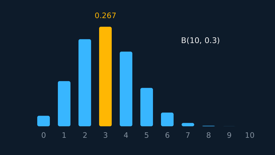
The three factors are: p to the power x for the successes, (1 − p) to the power n − x for the failures, and the binomial coefficient for the number of orders in which those successes can occur.
WORKED EXAMPLE
A point probability by hand
A biased coin lands heads with probability 0.3. It is flipped 10 times. Find the probability of exactly 3 heads.
P(X = 3) = ¹⁰C₃ × 0.3³ × 0.7⁷ = 120 × 0.027 × 0.0823543.
That multiplies to 0.267 (3 s.f.).
Check: np = 3, so P(X = 3) is expected to be the largest single probability in this distribution, which it is.
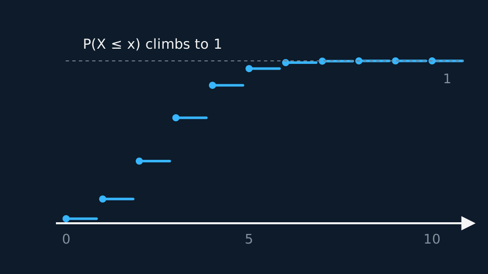
Cumulative probabilities come from the calculator's binomial cumulative function, which evaluates P(X ≤ x). Convert each inequality to that form first: P(X < 5) is P(X ≤ 4); P(X ≥ 7) is 1 − P(X ≤ 6); and P(3 ≤ X < 8) is P(X ≤ 7) − P(X ≤ 2). Since X is discrete, the strict and non-strict inequalities differ by one whole value.
ASSESSMENT FOCUS
- To check the model, state the conditions in this context: what one trial is, what counts as a success, and why p is constant.
- State X ~ B(n, p) before calculating.
- Write every inequality in ≤ form before using the calculator, and leave that conversion visible.
- Give probabilities to three significant figures unless the working produces an exact fraction.
CHECK YOURSELF
X ~ B(20, 0.15). Write P(X ≥ 5) in a form a calculator's cumulative function accepts, and state the value of P(X = 0) as a power.
Show a hint
At least five means not four-or-fewer.
Show the answer
P(X ≥ 5) = 1 − P(X ≤ 4).
P(X = 0) = 0.85²⁰, the probability that every trial is a failure.
Fixed n, two outcomes, constant p, independent trials. Only then is it binomial.
Point probabilities by the formula, everything else through ≤ and the cumulative function.
WORKBOOK
Printable practice for this topic: original exam-style questions with room to work, and a fully worked answer book. Free to use; please do not redistribute or sell.
Or read them with their worked answers on the binomial distribution questions page.
CHECK YOUR PROGRESS
Rate how confident you feel with each objective for this lesson. Ratings are saved in this browser, on this device, unless you sign in.
- Use a discrete probability distribution given as a table or as a formula, including finding an unknown constant.
- Recognise and name the discrete uniform distribution, and say why a given situation is or is not one.
- State and check the four conditions for X ~ B(n, p) to model a situation.
- Calculate P(X = x) from the formula and cumulative probabilities from a calculator.
- Convert “more than”, “at least” and “fewer than” into the ≤ form a calculator will accept.
Open the full revision checklist to see every objective in the course in one place.