Maths › Statistics › The normal distribution
The normal distribution
The normal distribution models continuous data that are approximately symmetric and bell-shaped. Calculate probabilities as areas under the curve, standardise values, and determine unknown parameters from stated probabilities.
Builds on The binomial distribution.
IN THIS TOPIC
- Use the shape and symmetry of X ~ N(μ, σ²), including the points of inflection at μ ± σ.
- Find probabilities and inverse-normal values with a calculator.
- Standardise with Z = (X − μ)/σ to find an unknown μ or σ from given probabilities.
- Approximate a binomial by a normal when n is large and p is near 0.5, applying a continuity correction.
- State when neither model suits the context.
COMMON MISCONCEPTION
About half of a normal population lies more than one standard deviation from the mean.
About 68% of a normal population lies within one standard deviation of the mean, so about 32% lies further out, roughly a third rather than a half. The matching figures are 95% within two standard deviations and 99.7% within three, for a distribution that is symmetric and bell-shaped about μ. Use them to check the size of a calculated probability.
The normal curve and when it applies
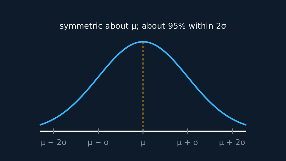
X ~ N(μ, σ²) says X is continuous, symmetric about its mean μ, with spread measured by its standard deviation σ. The curve's points of inflection are at μ ± σ, which allows σ to be read from a sketch. About 68% of values fall within one σ of the mean, 95% within two and 99.7% within three; use these figures to check the size of a calculated probability.
The normal distribution is not a default model for every continuous quantity. It applies to data that are approximately symmetric and bell-shaped; continuous distributions can also be skewed, bounded, multimodal or heavy-tailed, and a normal model then gives poor probabilities.
P(X = 40) is zero for a continuous variable: only intervals have non-zero probability, so P(X < 40) and P(X ≤ 40) are equal. A normal probability is an area under the curve, so sketch and shade the required region before calculating.
Areas from the calculator
WORKED EXAMPLE
A straightforward tail
Masses are modelled by X ~ N(50, 4²) in grams. Find the probability a mass exceeds 56 g.
Standardise first to see how big the answer should be: z = (56 − 50)/4 = 1.5, so this is the area beyond one and a half standard deviations.
The calculator gives P(X > 56) = 0.0668 (3 s.f.).
Check: the area beyond 1σ is about 16% and beyond 2σ about 2.5%, and 6.7% lies between those values, as expected for z = 1.5.
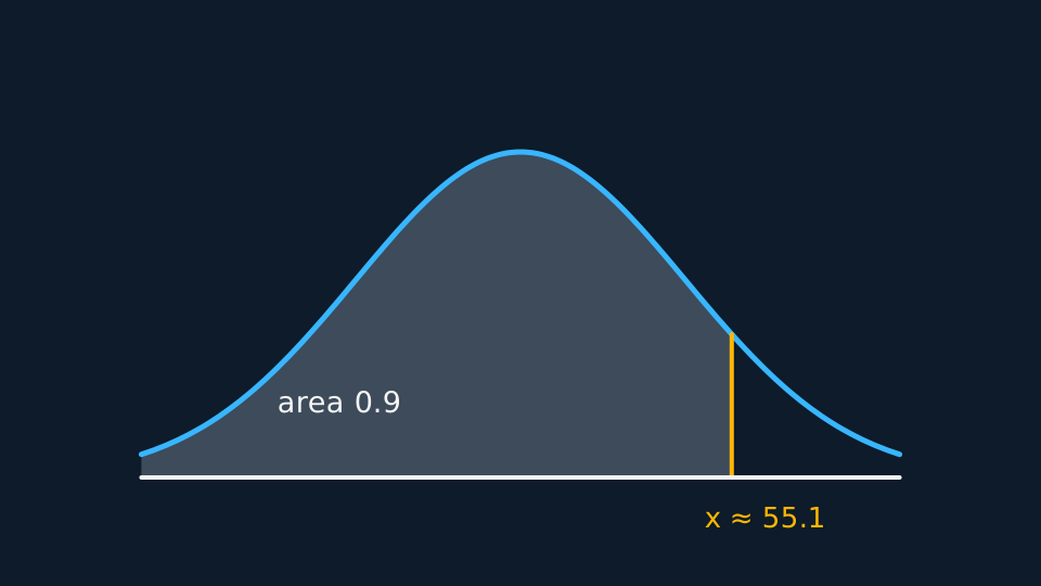
The inverse normal reverses that process, taking an area and returning a value. For P(X < x) = 0.9 with the model above, the calculator returns x ≈ 55.1 g. It takes the area to the left, so for the top 10% enter 0.9.
Finding μ or σ
When μ or σ is unknown, standardise first. Convert the given probability into a z-value using the inverse normal on N(0, 1), then solve the resulting equation for the unknown parameter.
WORKED EXAMPLE
An unknown standard deviation
X ~ N(30, σ²) and P(X > 35) = 0.02. Find σ.
P(Z > z) = 0.02 gives z = 2.0537 from the standard normal.
So (35 − 30)/σ = 2.0537, giving σ = 5/2.0537 = 2.43 (3 s.f.).
Check by working forwards: 35 is then about 2.05 standard deviations above 30, and the area beyond 2.05σ is about 2%.
Two unknown parameters need two given probabilities. Standardise both to obtain a pair of simultaneous equations in μ and σ.
Approximating a binomial
Summing a binomial with large n by hand is laborious, and when p is close to 0.5 the distribution is approximately symmetric and bell-shaped, so a normal distribution approximates it.
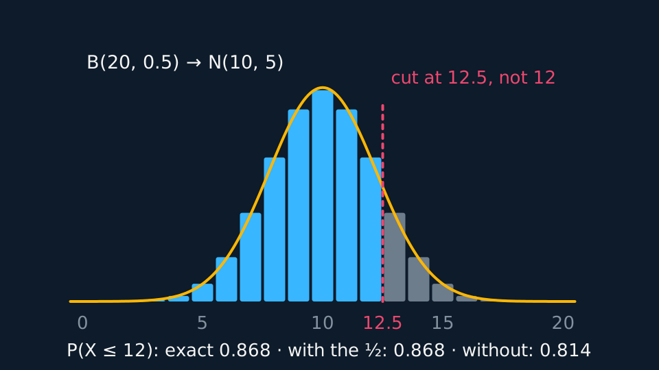
The approximation matches the mean and the variance. Because a discrete count is being replaced by a continuous variable, apply the continuity correction, extending each boundary by a half: P(X ≤ 60) becomes P(Y < 60.5), P(X ≥ 60) becomes P(Y > 59.5), and P(X = 60) becomes P(59.5 < Y < 60.5).
Describe the drawing
The twenty-one bars of B(20, 0.5) with the matching normal curve for N(10, 5) drawn over them, the bars up to twelve coloured and a dashed boundary line standing at twelve and a half: widened by the half-unit continuity correction the normal area is 0.868, agreeing with the exact binomial 0.868, while cutting at twelve would give only 0.814.
WORKED EXAMPLE
Using the approximation
X ~ B(150, 0.45). Use a suitable approximation to estimate P(X ≤ 60).
np = 67.5 and np(1 − p) = 37.125, so Y ~ N(67.5, 37.125) with σ = 6.09.
With the continuity correction, P(X ≤ 60) ≈ P(Y < 60.5), and z = (60.5 − 67.5)/6.09 = −1.149.
That gives 0.125 (3 s.f.). The exact binomial value is 0.1251, so the approximation agrees to 3 significant figures here.
State the conditions when using it: n large and p close to 0.5. State also when neither model is appropriate. A normal model assigns positive probability to every interval of values, negative ones included, so it is unsuitable for a quantity that cannot be negative and has a long right tail, such as rainfall or waiting time.
ASSESSMENT FOCUS
- Sketch and shade the required region before calculating, to fix which tail is wanted.
- The inverse normal takes the area to the left, so convert “the top 15%” into 0.85 before entering it.
- For an unknown parameter, show the standardising line Z = (X − μ)/σ before solving.
- Quote probabilities to 3 significant figures and z-values to at least 4, so that rounding does not affect the final answer.
- When using an approximation, name the approximating distribution, show the continuity correction and state the conditions under which it is used.
CHECK YOURSELF
X ~ N(μ, 6²) and P(X < 82) = 0.975. Use z = 1.96 to find μ.
Show a hint
Standardise, then solve for the one unknown.
Show the answer
(82 − μ)/6 = 1.96, so μ = 82 − 6 × 1.96 = 70.24, about 70.2.
Check: 82 sits nearly two standard deviations above 70.2, matching an area of 0.975.
The normal curve is symmetric about μ, with points of inflection at μ ± σ and about 95% of the distribution within 2σ of the mean.
Use a normal model only for data that are approximately symmetric and bell-shaped, and standardise with Z = (X − μ)/σ whenever a parameter is unknown.
WORKBOOK
Printable practice for this topic: original exam-style questions with room to work, and a fully worked answer book. Free to use; please do not redistribute or sell.
Or read them with their worked answers on the normal distribution questions page.
USED LATER IN
CHECK YOUR PROGRESS
Rate how confident you feel with each objective for this lesson. Ratings are saved in this browser, on this device, unless you sign in.
- Use the shape and symmetry of X ~ N(μ, σ²), including the points of inflection at μ ± σ.
- Find probabilities and inverse-normal values with a calculator.
- Standardise with Z = (X − μ)/σ to find an unknown μ or σ from given probabilities.
- Approximate a binomial by a normal when n is large and p is near 0.5, applying a continuity correction.
- State when neither model suits the context.
Open the full revision checklist to see every objective in the course in one place.