Maths › Further Statistics 1 › The Central Limit Theorem
The Central Limit Theorem
The Central Limit Theorem states that for independent, identically distributed observations from a population with finite variance, the sample mean is approximately normal for large n, whatever the shape of that population, with a standard error that falls in proportion to one over the square root of the sample size.
Builds on The normal distribution and The Poisson distribution.
IN THIS TOPIC
- State the Central Limit Theorem and the distribution it gives the sample mean.
- Compute probabilities for a sample mean or a sample total from a parent distribution meeting the theorem's conditions, for large enough n.
- Say what the theorem does not claim.
COMMON MISCONCEPTION
The sample mean can only be treated as normal when the population it comes from is itself normal.
For independent, identically distributed observations from a population of finite variance, the sample mean is approximately N(μ, σ²/n) for large n whatever the shape of that population, which may be skewed, discrete or bounded. The approximation describes the sampling distribution of the mean, not the observations, which keep the shape of the parent however much data is collected.
The sampling distribution of the mean
Take n independent observations from one population with mean μ and finite variance σ². For large n the sample mean is approximately normal, whatever shape that population has:
Pearson Edexcel 9FM0 formulae booklet: included, under Sampling distributions, which gives the sample mean as an unbiased estimator of μ with variance σ²/n and gives the standardised form as N(0, 1). The theorem itself has to be stated in words: for independent, identically distributed observations with finite variance, the sample mean is approximately normal for large n. The population may be skewed, discrete or bounded; the approximation applies to the distribution of the mean, not to the observations. The variance of the mean is σ²/n, so the standard error σ/√n falls with the square root of the sample size: quadrupling n halves it.
The same result runs on totals. Adding n independent observations gives a total that is approximately N(nμ, nσ²), which is often the quicker route when a question asks about a combined weight or a combined time.
Describe the drawing
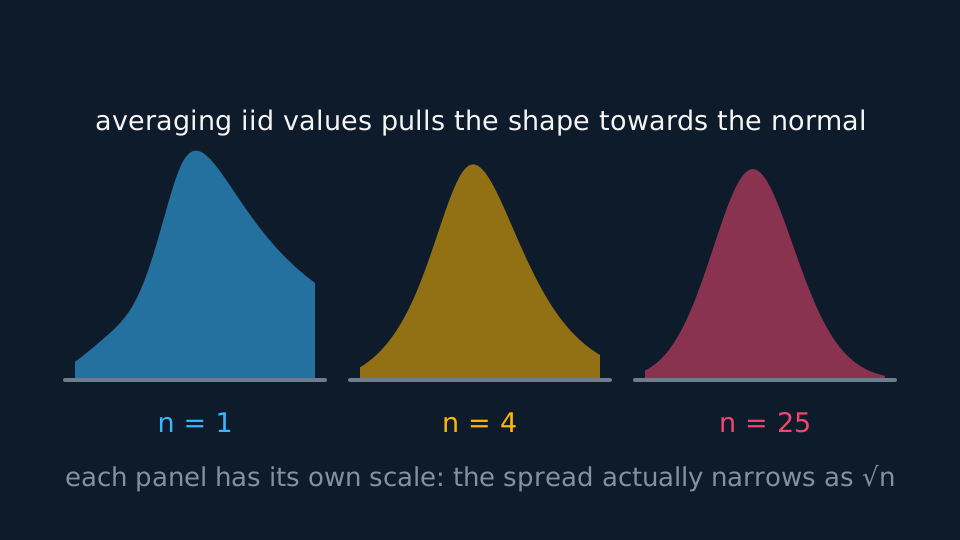
Three shaded distributions side by side, each drawn on its own scale. The first, for single observations, leans heavily to the right; the second, for means of four independent copies, is noticeably more even; the third, for means of twenty-five, is close to a symmetric bell. For independent, identically distributed values with finite variance, averaging straightens the shape while the true spread narrows as the square root of n.
WORKED EXAMPLE
A probability for a sample mean
A population has mean 50 and standard deviation 12, with unknown shape. For a sample of 36, find the probability the sample mean exceeds 53.
By the Central Limit Theorem, the mean is approximately N(50, 144/36), that is N(50, 4) with standard error 2.
z = (53 − 50)/2 = 1.5.
P(Z > 1.5) = 0.0668. Only the mean and standard deviation of the population entered the calculation; its shape did not, because n is large enough for the approximation.
Conditions and limitations
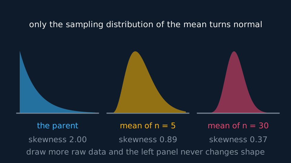
The theorem describes the sampling distribution of a sum or a mean, not the population. A skewed population stays skewed however large the sample grows, and a histogram of 500 raw observations shows that skew. Only the sampling distribution of the mean approaches a normal shape.
Describe the drawing
Three shaded density curves. The first is the exponential parent itself, piled against zero with skewness two, and it keeps that shape however many raw observations are drawn. The second is the distribution of the mean of five observations, already far less lopsided at skewness nought point eight nine; the third, for means of thirty, is close to a symmetric bell at nought point three seven. Averaging drives the mean's skewness towards zero as one over root n, while the parent never moves.
It is also an approximation with no fixed threshold. Textbooks offer n above 30 as a working rule, but the sample size required depends on the shape and tail behaviour of the population: a strongly skewed or heavy-tailed population needs more, a nearly symmetric one less. The conditions are that the observations are independent, identically distributed and drawn from a population with finite variance.
A biased sampling method is a separate problem. It may still produce an approximately normal sample mean, but centred on the mean of the population actually sampled rather than the target population. It therefore undermines the inference rather than the theorem itself.
GUIDED PRACTICE
Spotting the misuse
A student writes: 'The sample of 40 lifetimes came from an exponential population, so by the Central Limit Theorem the lifetimes are approximately normal.' Correct the statement.
Show the working
The lifetimes themselves stay exponential and stay skewed. Sample size does not change the parent.
What is approximately normal is the mean of the 40 lifetimes, with variance σ²/40, and the total of the 40, with variance 40σ².
A probability about one lifetime needs the exponential model; only a probability about the average may use the normal one.
Sample size and standard error
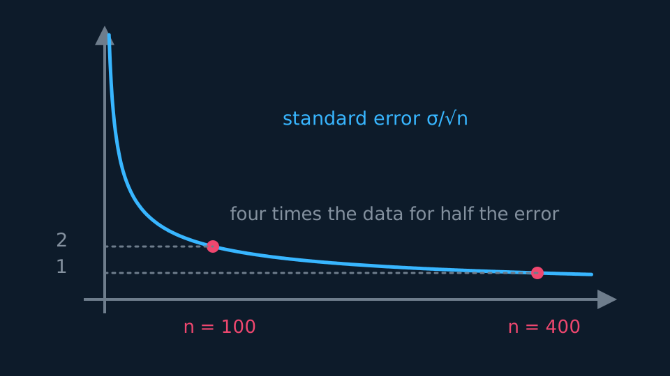
Because the standard error is σ/√n rather than σ/n, halving the spread of the sample mean requires four times the data. This is why the sample size needed climbs steeply as the required margin narrows.
GUIDED PRACTICE
Sizing a sample
A population has standard deviation 20. How large must a sample be for the standard error of the mean to be at most 2?
Show the working
Standard error = 20/√n ≤ 2, so √n ≥ 10.
n ≥ 100.
Reducing the standard error to 1 would need n ≥ 400. Halving the error quadruples the sample.
ASSESSMENT FOCUS
- Quote the conclusion as a distribution, with mean μ, variance σ²/n, approximately normal.
- Divide the variance by n, not the standard deviation. The standard error is σ/√n.
- Say 'approximately' and state that n is large. The theorem gives an approximation, and a complete answer says so.
- For a total rather than a mean, use N(nμ, nσ²) and check which the question asked for.
CHECK YOURSELF
A distribution has mean 30 and variance 100. Write down the approximate distribution of the mean of a sample of 25, and of the total of the 25.
Show a hint
Divide the variance by n for the mean; multiply by n for the total.
Show the answer
The mean is approximately N(30, 4), with standard error 2. The total is approximately N(750, 2500), with standard deviation 50.
For large n, with independent identically distributed observations of finite variance, the sample mean is approximately N(μ, σ²/n) and the total approximately N(nμ, nσ²), whatever the shape of the population.
The population distribution itself is unchanged by sample size, and the standard error σ/√n needs four times the data for half the spread.
WORKBOOK
Printable practice for this topic: original exam-style questions with room to work, and a fully worked answer book. Free to use; please do not redistribute or sell.
Or read them with their worked answers on the Central Limit Theorem questions page.
USED LATER IN
CHECK YOUR PROGRESS
Rate how confident you feel with each objective for this lesson. Ratings are saved in this browser, on this device, unless you sign in.
- State the Central Limit Theorem and the distribution it gives the sample mean.
- Compute probabilities for a sample mean or a sample total from a parent distribution meeting the theorem's conditions, for large enough n.
- Say what the theorem does not claim.
Open the full revision checklist to see every objective in the course in one place.