Maths › Further Statistics 2 › Confidence intervals and tests with the t-distribution
Confidence intervals and tests with the t-distribution
Estimating the variance from the same small sample adds uncertainty, and the t-distribution accounts for it. It has heavier tails than the normal, so intervals built from it are wider. Apply it to the one-sample, paired and two-sample cases, stating the normality and equal-variance assumptions each needs.
Builds on Comparing two normal means and Estimators, standard error and confidence intervals and Hypothesis testing: correlation and the normal.
IN THIS TOPIC
- Carry out a one-sample t test and build the matching confidence interval.
- Recognise paired data from how it was collected and reduce it to a single sample of differences.
- Pool two sample variances and run a two-sample t test.
- State the assumptions each version of the test requires.
COMMON MISCONCEPTION
With a sample of 12 you should use z = 1.96 for a 95% interval, since the sample mean is normal.
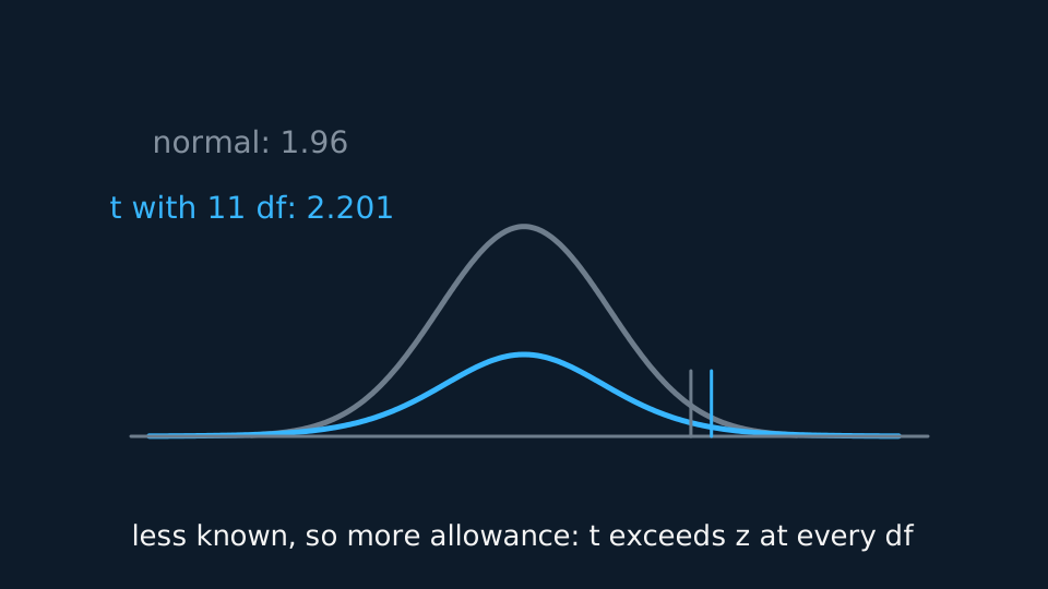
With σ estimated by s from the same small sample, the standardised mean follows t on n − 1 degrees of freedom, whose tails are heavier than the normal's. On the 11 degrees of freedom a sample of 12 gives, the two-tailed 5% value is 2.201 rather than 1.96, so using 1.96 makes every interval too narrow and every test too willing to reject. The two converge as n grows.
The t-distribution when the variance is estimated
When σ is unknown and estimated by s from the same small sample, the standardised mean stops following the normal distribution:
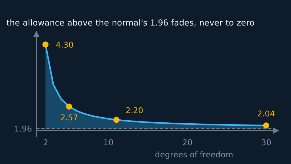
Pearson Edexcel 9FM0 formulae booklet: included, under Sampling distributions, where it is also given for matched pairs, with percentage points of t tabulated. The t distribution is symmetric and centred at zero like the normal, but its tails are heavier, so the value cutting off 2.5% sits further out. On 11 degrees of freedom that value is 2.201 against 1.96 for the normal. Using 1.96 anyway makes every interval too narrow and every test too willing to reject. As n grows the two converge, and beyond about 30 the difference stops mattering much.
The exact small-sample result still rests on normality, and each version of the test names its own population: the measurements for a one-sample test, the within-pair differences for a paired test, and both populations for the pooled test.
WORKED EXAMPLE
A one-sample t test and interval
A sample of 12 has mean 25.4 and s = 3.2. Test at 5% whether the population mean exceeds 23, and give a 95% interval for it.
Standard error = 3.2/√12 = 0.924. t = (25.4 − 23)/0.924 = 2.60 on 11 degrees of freedom.
The one-tailed 5% critical value is 1.796, and 2.60 exceeds it, so reject H₀. There is evidence that the mean exceeds 23.
The interval is two-sided, so it takes the two-tailed value 2.201: 25.4 ± 2.201 × 0.924 gives (23.37, 27.43).
Pair an interval with a test only when the tail areas agree. A 95% two-sided interval is the two-tailed 5% test, so this one missing 23 says the two-tailed test rejects μ = 23 as well, which is a different test from the one-tailed test above. The one-tailed 5% test pairs with the one-sided 95% bound, 25.4 − 1.796 × 0.924 = 23.74, or with the 90% two-sided interval (23.74, 27.06). Both put 23 outside, which is the agreement the duality actually promises.
So the pairing runs 95% two-sided interval with 5% two-tailed test, 90% two-sided interval with 5% one-tailed test. Reading a 95% two-sided interval as a 5% one-tailed test halves the tail area you meant to use and quietly turns the test into a 2.5% one.
Paired data
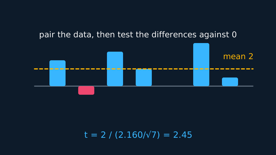
When each reading in one sample has a natural partner in the other, before and after on the same subject for instance, subtract within pairs and test the single sample of differences against zero. The degrees of freedom come from the number of pairs, not the number of readings, so seven pairs give 6.
Pairing removes the variation between subjects, which is usually the largest source of noise in the data. When that between-subject variation is real, a paired design detects smaller effects than an unpaired one built from the same number of readings; when the pairing is uninformative, it spends degrees of freedom for nothing. Treating paired data as two independent samples discards that advantage and uses a larger standard error than the design requires.
Which design you have is a property of the data rather than of the test, so settle it before choosing anything. A paired sample arrives in a fixed order with a partner for each reading, the same subject measured twice or two subjects matched on whatever else would differ, and the two lists are the same length. An unpaired one is two independent groups whose sizes need not agree and whose orders carry no information. Samples of different sizes settle the question at once; so does finding that shuffling one list would change nothing. The same reading of the data picks the paired or the two-sample form of whichever test follows.
WORKED EXAMPLE
Before and after
Seven athletes are timed before and after a training programme. The improvements in seconds are 3, 1, 4, 0, 2, 5, −1. Test at 5% in two tails whether the programme changes performance.
H₀: the mean difference is 0; H₁: it is not 0. Work with the seven differences alone.
Their mean is 14/7 = 2 and their sum of squares is 56, so Sdd = 56 − 14²/7 = 28 and s² = 28/6 = 4.67, giving s = 2.160.
Standard error = 2.160/√7 = 0.8165, so t = 2/0.8165 = 2.449 on 6 degrees of freedom.
The two-tailed 5% critical value is 2.447. Since 2.449 exceeds it, reject H₀, but only just. There is evidence at the 5% level that the programme changes performance. The margin is two thousandths, so a single reading a second smaller could send the verdict the other way, and an answer here should say the result is marginal.
Two independent samples and a pooled variance
For two genuinely independent samples drawn from normal populations with a common unknown variance, pool the two estimates in proportion to their degrees of freedom:
Pearson Edexcel 9FM0 formulae booklet: the pooled estimate and the two-sample t statistic that uses it are both included. The test statistic then divides the difference of the means by s√(1/n1 + 1/n2), on n1 + n2 − 2 degrees of freedom. Averaging the two variances instead of weighting them gives the wrong answer whenever the samples differ in size. The assumption of equal variances is exactly what an F test checks, so the two topics belong together and an exam can ask you to run one before the other.
Pooling is worth the assumption because of what it gains: the combined n1 + n2 − 2 degrees of freedom pull the critical value down towards the normal's, so the same data give a sharper test than either sample could manage alone.
Describe the drawing
A falling cyan curve of the t critical value against the degrees of freedom, starting at four point three on two degrees of freedom, passing two point two zero at eleven, and flattening towards a dashed line at one point nine six. The shaded gap between curve and line is the extra allowance for estimating the variance, and it shrinks at every step without ever quite closing.
GUIDED PRACTICE
Pooling two samples
Sample 1: n = 8, mean 42, s = 5. Sample 2: n = 10, mean 38, s = 4. Test at 5% in two tails whether the means differ, given a critical value of 2.120.
Show the working
Pooled variance = (7 × 25 + 9 × 16)/16 = 319/16 = 19.94, so s = 4.465.
Standard error = 4.465 × √(1/8 + 1/10) = 4.465 × 0.4743 = 2.118.
t = 4/2.118 = 1.89 on 16 degrees of freedom.
Since 1.89 < 2.120, do not reject H₀. There is insufficient evidence at the 5% level that the population means differ.
ASSESSMENT FOCUS
- Count the degrees of freedom before opening the tables: n − 1, the number of pairs minus 1, or n₁ + n₂ − 2 when pooling.
- Look for the word 'paired' or a natural pairing in the data. The unpaired test on paired data throws information away.
- Two samples of different sizes rule pairing out. Two lists of the same length prove nothing on their own, so name the partner each reading has.
- Pool by weighting each sample variance by its own degrees of freedom, never by averaging the two.
- State the assumptions: normality of the relevant population, which for a paired test means the differences themselves, and equal variances for the pooled test.
- Halve the level for each tail of a two-tailed t test, exactly as with z.
- Match the tails before using an interval as a test. A 95% two-sided interval answers the two-tailed 5% test; a 5% one-tailed test needs the one-sided 95% bound, or the 90% two-sided interval.
- Read critical values straight from the tables at full accuracy. On a borderline case the third decimal place decides it.
CHECK YOURSELF
A sample of 9 has mean 51 and s = 6. Find the test statistic for H₀: μ = 48 and state the degrees of freedom.
Show a hint
Standard error first, then divide.
Show the answer
Standard error = 6/√9 = 2, so t = (51 − 48)/2 = 1.5 on 8 degrees of freedom.
With σ estimated from the sample, use t on n − 1 degrees of freedom: heavier tails than the normal, so wider intervals.
Paired data becomes one sample of differences; independent samples with a common variance use the pooled s² on n₁ + n₂ − 2 degrees of freedom.
Paired or unpaired is decided by how the data were collected, not by the test: equal-length lists with a partner for each reading are paired, and samples of different sizes are not.
WORKBOOK
Printable practice for this topic: original exam-style questions with room to work, and a fully worked answer book. Free to use; please do not redistribute or sell.
Or read them with their worked answers on the confidence intervals and tests with the t-distribution questions page.
CHECK YOUR PROGRESS
Rate how confident you feel with each objective for this lesson. Ratings are saved in this browser, on this device, unless you sign in.
- Carry out a one-sample t test and build the matching confidence interval.
- Recognise paired data from how it was collected and reduce it to a single sample of differences.
- Pool two sample variances and run a two-sample t test.
- State the assumptions each version of the test requires.
Open the full revision checklist to see every objective in the course in one place.