Maths › Statistics › Hypothesis testing: correlation and the normal
Hypothesis testing: correlation and the normal
Apply the hypothesis-testing procedure to two further situations: whether a sample correlation coefficient is evidence of correlation in the population, and whether the mean of a normal population with known variance has changed. Each uses a different distribution under the null hypothesis.
Builds on Hypothesis testing with the binomial and Correlation and regression.
IN THIS TOPIC
- Test H₀: ρ = 0 against a critical value read from the table, using the right column for the number of tails.
- Use the fact that the mean of n observations of N(μ, σ²) is N(μ, σ²/n).
- Carry out a hypothesis test for the mean of a normal distribution with known σ, concluding in context.
- Define the p-value as the probability, if H₀ is true, of a result at least as extreme as the one observed, and say what it is not.
COMMON MISCONCEPTION
The sample mean of n readings has the same standard deviation as a single reading.
The mean of n independent observations of N(μ, σ2) is itself normal, with the same mean μ and standard deviation σ/√n. Averaging 25 independent readings therefore divides the standard deviation by five, and σ/√n is the divisor when standardising in a test about a normal mean. Dividing by n instead gives incorrect z-values.
Testing a correlation coefficient
A sample can show apparent correlation when the population correlation is zero, so the test asks whether the sample value of r is too large to be attributed to sampling variation. The hypotheses are stated in terms of ρ, the population correlation coefficient: test H₀: ρ = 0 against H₁: ρ > 0, ρ < 0 or ρ ≠ 0. State the hypotheses in ρ, not in r.
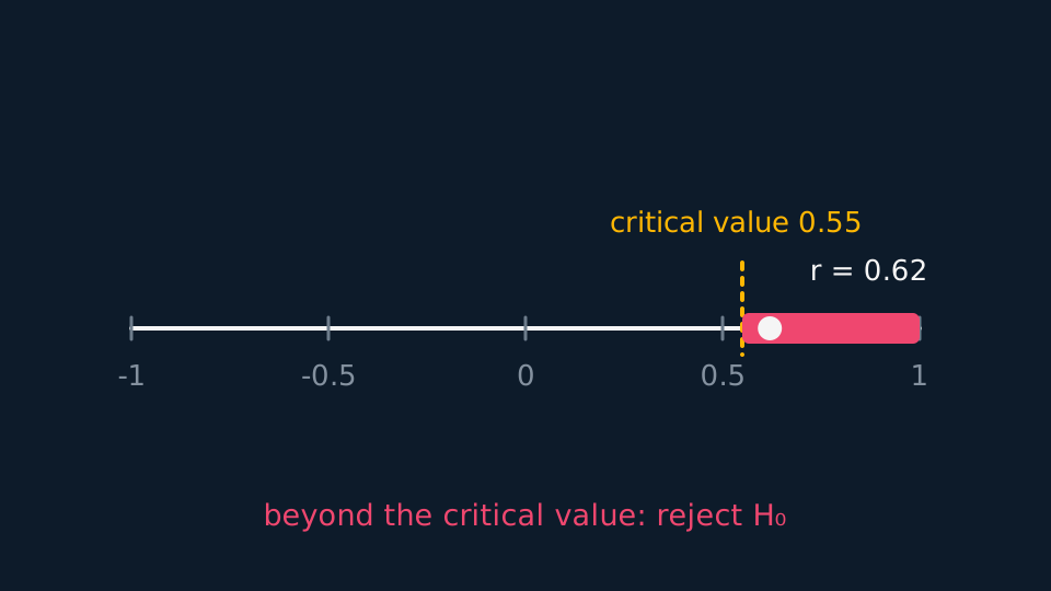
The table of critical values is indexed by sample size and by one-tail probability, so select the column that matches the number of tails. A one-tailed test at 5% uses the 0.05 column; a two-tailed test at 5% uses the 0.025 column, because the significance level is divided between the tails.
The test is then a single comparison. For H₁: ρ > 0, reject H₀ when r exceeds the positive critical value. For H₁: ρ < 0, reject H₀ when r is less than the corresponding negative value. Only the two-tailed test compares |r| with the critical value. With n = 20 and r = 0.48 against H₁: ρ ≠ 0 at 5%, the table gives 0.4438, and 0.48 > 0.4438, so at the 5% significance level reject H₀ and conclude that there is sufficient evidence of correlation between the two named variables. This test assesses linear association; it does not establish causation.
The sample mean's distribution
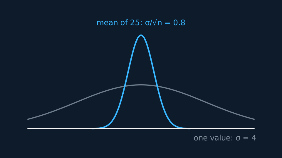
The mean of n independent observations of N(μ, σ²) is itself normal, with the same mean μ and standard deviation σ/√n. That standard deviation is the divisor used when standardising in a test about a normal mean; dividing by n rather than √n gives incorrect z-values.
The formulae booklet prints this result in its standardised form: for a random sample of n observations from N(μ, σ²), the sample mean minus μ, divided by σ/√n, is N(0, 1). Be able to write down the distribution N(μ, σ²/n) and then standardise it.
Testing a normal mean
WORKED EXAMPLE
Has the machine drifted?
Bags from a machine have masses N(μ, 4²) grams. The machine is set to μ = 30. A sample of 25 bags has mean 31.6 g. Test at the 5% level whether the mean has increased.
H₀: μ = 30, H₁: μ > 30. Under H₀ the sample mean is N(30, 4²/25), standard deviation 4/5 = 0.8.
z = (31.6 − 30)/0.8 = 2.0, and P(Z ≥ 2.0) = 0.0228.
0.0228 < 0.05, so at the 5% significance level reject H₀ and conclude that there is sufficient evidence that the mean mass has increased.
Check: 31.6 is two standard deviations of the sample mean above 30, and the area beyond z = 2 is about 2.3%, consistent with the p-value obtained.
The 0.0228 is the p-value: the probability, if H₀ is true, of a result at least as extreme as the one observed, which here means a sample mean of 31.6 g or more. It is compared with the significance level, and H₀ is rejected when it is smaller. It is not the probability that H₀ is true, which no test gives; it is a probability calculated assuming H₀. In a two-tailed test a sample mean as far below 30 would count as just as extreme, so the tail probability is doubled before the comparison, or compared with half the level.
The critical-value method gives the same decision. At the 5% level, reject H₀ when z > 1.6449 for a one-tailed test, or when |z| > 1.96 for a two-tailed test. As with the binomial test, a two-tailed test divides the significance level between the tails, and the conclusion is stated in the same form.
ASSESSMENT FOCUS
- Correlation tests: hypotheses in ρ, comparison against the table's critical value, conclusion naming both variables.
- Select the table column by the number of tails: a two-tailed test at 5% uses the 0.025 column.
- For a normal-mean test, write the distribution of the sample mean, with standard deviation σ/√n, before standardising.
- The wording fixes the number of tails: “changed” is two-tailed, “increased” or “decreased” is one-tailed.
- State the conclusion in context: reject or do not reject H₀, at the stated significance level, about the named quantity.
CHECK YOURSELF
Readings are N(μ, 9) and H₀ sets μ = 50. A sample of 36 has mean 49.2. Find the z-value for testing H₁: μ < 50.
Show a hint
The sample mean's standard deviation is σ/√n.
Show the answer
σ/√n = 3/6 = 0.5.
z = (49.2 − 50)/0.5 = −1.6.
Correlation: hypotheses in ρ, and compare the sample r against the table value for the right number of tails.
The mean of n independent readings has distribution N(μ, σ²/n), so standardise with σ/√n.
WORKBOOK
Printable practice for this topic: original exam-style questions with room to work, and a fully worked answer book. Free to use; please do not redistribute or sell.
Or read them with their worked answers on the hypothesis testing: correlation and the normal questions page.
USED LATER IN
CHECK YOUR PROGRESS
Rate how confident you feel with each objective for this lesson. Ratings are saved in this browser, on this device, unless you sign in.
- Test H₀: ρ = 0 against a critical value read from the table, using the right column for the number of tails.
- Use the fact that the mean of n observations of N(μ, σ²) is N(μ, σ²/n).
- Carry out a hypothesis test for the mean of a normal distribution with known σ, concluding in context.
- Define the p-value as the probability, if H₀ is true, of a result at least as extreme as the one observed, and say what it is not.
Open the full revision checklist to see every objective in the course in one place.