Maths › Further Pure 2 › Functions of two variables
Functions of two variables
A partial derivative differentiates with respect to one variable while holding the other fixed. The gradient gives the linear change and determines the tangent plane at a differentiable point. At a stationary point, use the Hessian test when it is decisive and use a direct or higher-order argument when it is not.
Builds on Tangents, turning points and curve behaviour and Determinants and inverses.
IN THIS TOPIC
- Read z = f(x, y) as a surface, and move between that form and an implicit g(x, y, z) = c.
- Carry the same algebra to more than two variables, and the same reading to trigonometric, logarithmic and exponential rules.
- Sketch sections z = f(a, y) and z = f(x, b), and contours c = f(x, y), and relate both to the surface.
- Find first, second and mixed partial derivatives in both notations, and state the condition under which the mixed derivatives agree.
- Locate stationary points by solving fx = 0 and fy = 0 together, and describe maxima, minima and saddle points.
- Classify a stationary point by the sign of the Hessian determinant, and say when the test gives no verdict.
- Write down the tangent plane to a surface at a point where the function is differentiable.
- Use the tangent plane as a linear approximation to the function near the point of contact, and compare the estimate with the exact value.
COMMON MISCONCEPTION
If both partial derivatives vanish at a point, the surface has a maximum or a minimum there, just as a curve would.
A surface has a third possibility with no counterpart on a curve. At a saddle point it rises along one direction and falls along another, as z = x² − y² does at the origin, where both partial derivatives vanish. The determinant H = fxxfyy − (fxy)2 decides: negative means a saddle, positive a minimum or a maximum by the sign of fxx, and H = 0 leaves the test inconclusive.
Heights above the plane
A function of two variables takes a point (x, y) of the plane and returns a single number. Call that number z and the rule reads z = f(x, y). Plotting the point (x, y, z) for one input pair after another sweeps out a surface in three dimensions, with the plane as a floor and f as the height above it. Everything below is a way of reading that surface: slicing it, measuring its slope, and finding where it levels off.
The same surface can be written implicitly instead, as g(x, y, z) = c, with the three letters treated alike and z no longer the subject. Moving between the two forms is usually possible, and doing it can reveal that one implicit equation is carrying more than one explicit function.
WORKED EXAMPLE
One surface written two ways
The sphere x2 + y2 + z2 = 25 is given implicitly. Write it explicitly, and say which points of the plane the description reaches.
Rearranging gives z2 = 25 − x2 − y2, so z = ±√(25 − x2 − y2).
The positive root is the upper hemisphere and the negative root the lower, so one implicit equation holds two explicit functions, neither of them the whole sphere.
A point (x, y) has a height only when x2 + y2 ≤ 25. At (3, 4) both roots give z = 0, which is the equator; at the origin they give z = ±5, the two poles.
Reading the domain is part of reading the surface. A standard example is z = x/y, which has no value anywhere on the line y = 0, so this surface has a gap along a whole line of the plane rather than at one point. A rule that divides or takes a root needs a line saying where it applies.
Nothing in the definition holds the count at two. The volume of a box, V(x, y, z) = xyz, takes three inputs and obeys the same algebra: hold two of them still and differentiate in the third, so that Vx = yz, the area of the face that moves as the width grows. What is lost is the picture, since the graph of a function of three variables would need four dimensions. Nor are powers of x and y the only ingredients. Surfaces built from trigonometric, logarithmic and exponential expressions, such as z = e2x sin y or z = ln(xy), are handled by the rules below without change.
Sections and contours
Two families of curves make a surface readable, and both come from holding something fixed. Fix an input and you get a section: putting x = a leaves z = f(a, y), a curve in the vertical plane x = a, and putting y = b leaves z = f(x, b). Fix the output instead and you get a contour: setting f(x, y) = c leaves a curve in the plane of the inputs, joining the points at height c. A walker's map is drawn from contours; a slice through a loaf is a section.
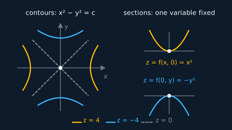
WORKED EXAMPLE
Slicing z = x² − y² both ways
For z = x2 − y2, find the sections along y = 0, along x = 0 and along x = 2, and the contours at z = 4, z = 0 and z = −4.
Along y = 0 the rule reduces to z = x2, a parabola opening upwards. Along x = 0 it reduces to z = −y2, the same parabola turned over. Along x = 2 it is z = 4 − y2, that downward parabola lifted to a vertex at height 4.
The contour at z = 4 is x2 − y2 = 4, a hyperbola with vertices at (±2, 0). At z = −4 it is y2 − x2 = 4, the same shape turned through a right angle, with vertices at (0, ±2).
At z = 0 the equation factorises as (x − y)(x + y) = 0, so the contour is the pair of lines y = x and y = −x. A contour that crosses itself is worth noticing: the surface is level in two directions at once there, and that crossing point turns out to be a saddle.
Contours crowd together where the surface is steep and spread out where it is flat, which is why a map with closely spaced lines promises a hard climb. Sections carry the same information one slice at a time, and a question that asks for a sketch of a surface is usually asking for two or three of one family, not for a drawing in perspective.
Differentiating one variable at a time
To differentiate a function of two variables, pick a variable and treat the other as a constant. What comes out is a partial derivative. Differentiating with respect to x measures how the height changes as you walk parallel to the x-axis, which is the gradient of the section along that fixed value of y. The partial derivative and the section are one idea seen twice.
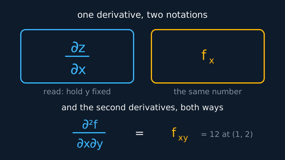
Two notations are in use. The function form writes fx and fy. The Leibniz form writes a fraction whose d is curled, one curl above and one below. Second derivatives follow the pattern: fxx differentiates twice with respect to x, fyy twice with respect to y, and the mixed derivative fxy once with respect to each.
State the convention used for subscripts: here fxy means differentiate first with respect to x, then y. The Leibniz fraction lists the two variables in the opposite order, so the same derivative appears written both ways.
If the relevant second partial derivatives are continuous near the point, fxy = fyx, which is the mixed derivative theorem. Under that hypothesis the order of differentiation does not matter, and computing both orders checks the arithmetic: two orders that disagree mean one of the four differentiations is wrong. Without continuity the two need not agree.
WORKED EXAMPLE
Five derivatives from one rule
For f(x, y) = x3y2 + 4x − y5, find the first and second partial derivatives, and evaluate them at (1, 2).
Holding y constant, fx = 3x2y2 + 4. Holding x constant, fy = 2x3y − 5y4.
Differentiating again: fxx = 6xy2, fyy = 2x3 − 20y3, and fxy = 6x2y from either order of differentiation.
At (1, 2): fx = 12 + 4 = 16 and fy = 4 − 80 = −76.
And fxx = 24, fyy = 2 − 160 = −158, fxy = 12. The two mixed derivatives agreeing is the check that the second round of differentiation is sound.
WORKED EXAMPLE
The same rules beyond powers
Find both first partial derivatives of f(x, y) = e2x sin y + ln(xy) for x > 0 and y > 0, and confirm that the mixed second derivatives agree.
Splitting the logarithm first is worth a line: ln(xy) = ln x + ln y, after which each piece depends on one variable only.
fx = 2e2x sin y + 1/x, since sin y is a constant multiplier while x moves. fy = e2x cos y + 1/y.
Differentiating fx with respect to y gives 2e2x cos y, because 1/x is now the constant. Differentiating fy with respect to x gives 2e2x cos y as well, so the theorem holds here as it should.
Where the surface levels off
A curve is stationary where its one derivative vanishes. A surface has two derivatives to make vanish, and a stationary point needs both at once: fx = 0 and fy = 0 at the same point. Setting one of them to zero on its own describes a curve in the plane rather than a point, so the two are solved as a simultaneous pair and each candidate is put back into both.
Three cases account for the stationary points met in this course. A local maximum is a peak, with the surface below the point in each direction away from it. A local minimum is a bowl. A saddle point is the shape with no counterpart on a curve: the surface rises along one direction through the point and falls along another, so the same point is a highest point one way and a lowest point the other. The surface z = x2 − y2 at the origin is the standard example, and its level contour crossing itself was the first sign of it.
Those three do not exhaust every possibility. The surface z = x2 is stationary at every point of the line x = 0 and is flat along that line, so no point of it is an isolated peak, bowl or saddle. Cases of that kind are exactly the ones the test below leaves undecided.
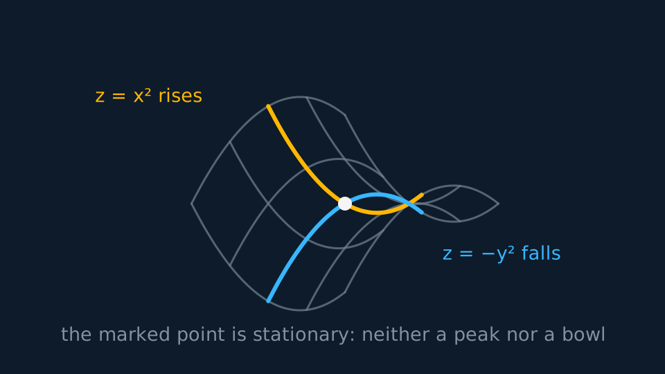
Decision Mathematics uses the words saddle point for a different object: the entry of a pay-off matrix at which the row maximin and the column minimax agree. The two share a shape, largest one way and smallest the other, but one is an entry in a table of numbers and the other a point of a surface, and no result about either carries across to the other.
WORKED EXAMPLE
Both derivatives at once
Find the stationary points of f(x, y) = x3 + y3 − 3xy.
fx = 3x2 − 3y and fy = 3y2 − 3x. Setting both to zero gives y = x2 and x = y2.
Substituting the first into the second gives x = x4, so x4 − x = 0 and x(x3 − 1) = 0, leaving x = 0 or x = 1.
Then y = x2 gives the two points (0, 0) and (1, 1), at heights f(0, 0) = 0 and f(1, 1) = 1 + 1 − 3 = −1.
Both were found with no picture of the surface, and neither has been classified. That is the next section's work.
The Hessian test
The second derivatives settle which of the three shapes a stationary point has. Assemble them into the Hessian matrix, with fxx and fxy along the first row and fyx and fyy along the second, and take its determinant. Where the mixed derivatives agree, that determinant is H = fxxfyy − (fxy)2, with the last term squared.
| The determinant H | Then look at | The stationary point is |
|---|---|---|
| H > 0 | fxx > 0 | a local minimum |
| H > 0 | fxx < 0 | a local maximum |
| H < 0 | nothing further | a saddle point |
| H = 0 | nothing available | not settled: the test is inconclusive |
Read the table in that order. The sign of H decides first, separating the two definite cases from the saddle; only once H is positive does fxx come into it, and then it says which way up. If H = 0 the test is inconclusive and higher-order or direct analysis is required. Both z = x4 + y4 and z = x4 − y4 have H = 0 at the origin: the first has a minimum there and the second a saddle, so the value of H alone cannot separate them.
WORKED EXAMPLE
Classifying the two points
Classify the stationary points (0, 0) and (1, 1) of f(x, y) = x3 + y3 − 3xy.
From fx = 3x2 − 3y and fy = 3y2 − 3x come fxx = 6x, fyy = 6y and fxy = −3, so H = 36xy − 9.
At (0, 0), H = −9, which is negative, so the origin is a saddle point.
At (1, 1), H = 36 − 9 = 27, which is positive, and fxx = 6 is positive as well, so (1, 1) is a local minimum, at height −1.
A ring of points round each one confirms the verdicts: close to (1, 1) the surface stays above −1 the whole way round, while close to the origin it takes both signs.
Tangent planes
A curve has a tangent line at a point; a surface has a tangent plane. Build it from the two sections through the point. The section along y = b has gradient fx(a, b) there, the section along x = a has gradient fy(a, b), and the plane containing both of those tangent lines is the tangent plane at (a, b, f(a, b)).
In symbols it is z = f(a, b) + (x − a)fx(a, b) + (y − b)fy(a, b). That is the two-variable version of y = f(a) + (x − a)f′(a), with one term for each direction: start at the height of the point, then add what each step away from it gains or loses. The formula assumes f is differentiable at (a, b). The existence of the two partial derivatives there is not by itself enough, since a function can have both partial derivatives at a point and no tangent plane.
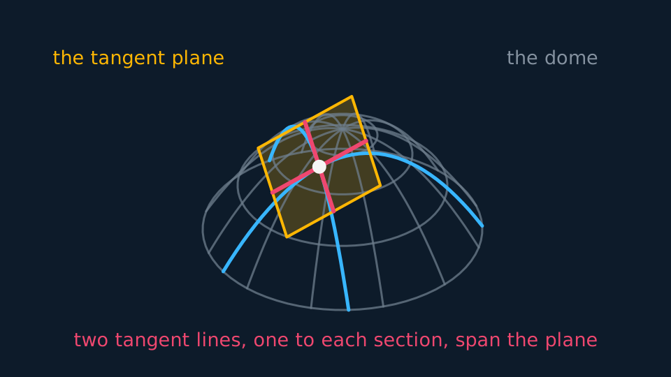
WORKED EXAMPLE
A tangent plane at a point
Find the tangent plane to z = x2y + 2y2 at the point where x = 1 and y = 2.
The height first: f(1, 2) = 2 + 8 = 10, so the point is (1, 2, 10).
Then the slopes: fx = 2xy, worth 4 there, and fy = x2 + 4y, worth 9 there.
The plane is z = 10 + 4(x − 1) + 9(y − 2), which tidies to z = 4x + 9y − 12.
Check it. At (1, 2) the plane gives 4 + 18 − 12 = 10, the right height. A short step to (1.01, 2.01) gives 10.130 from the plane and 10.1306 from the surface, and a gap of 0.0006 on a step of 0.01 is second order in the step, which is what a tangent promises.
That check is the tangent plane's second use. Near the point of contact the plane and the surface are close, so f(a + h, b + k) ≈ f(a, b) + hfx(a, b) + kfy(a, b) is a linear approximation to the function, the two-variable version of f(a + h) ≈ f(a) + hf′(a). It is the way to estimate a value from a measured point and measured rates of change, and its error grows with the square of the step, so it is only to be trusted close in.
Estimating f(1.1, 1.9) from the plane above gives 4.4 + 17.1 − 12 = 9.5, against the exact 1.21 × 1.9 + 2 × 3.61 = 9.519: the estimate is 0.019 low on a step of about 0.14, and the second derivatives, 2y, 2x and 4, supply a second-order correction of 0.020, with the remaining 0.001 third order in the step.
At a stationary point both slopes are zero, so the formula collapses to z = f(a, b) and the tangent plane is horizontal. That is the surface's version of a curve's flat tangent, and it holds at a saddle as readily as at a peak or a bowl, which is why a horizontal tangent plane says nothing about which of the three you have and the Hessian is still wanted.
GUIDED PRACTICE
Find it, classify it, then flatten it
For f(x, y) = x2 + xy + y2 − 3x, find the stationary point, classify it, and write down the tangent plane there.
Show the working
fx = 2x + y − 3 and fy = x + 2y. The second gives x = −2y, and substituting into the first gives −4y + y − 3 = 0, so y = −1 and x = 2.
fxx = 2, fyy = 2 and fxy = 1, so H = 4 − 1 = 3. That is positive and fxx is positive, so (2, −1) is a local minimum, at height 4 − 2 + 1 − 6 = −3.
Both partial derivatives vanish there, so the tangent plane is the horizontal plane z = −3.
ASSESSMENT FOCUS
- Differentiate with respect to one variable while the other is held constant, and write f_x or the curly-d fraction rather than dy/dx.
- State the subscript convention before using it: f_xy here means differentiate with respect to x, then y.
- A stationary point needs both partial derivatives to vanish, so solve the two equations as a simultaneous pair and check each answer in both.
- Write the Hessian determinant as f_xx f_yy − (f_xy)², with the mixed derivative squared.
- Take the sign of H first and only then look at f_xx; if H is zero, state that the test is inconclusive and examine the surface directly.
- Name the type in words as well as by the inequality: local maximum, local minimum, saddle point.
- For a tangent plane, work out f, f_x and f_y at the point before substituting into the formula, and say that f is differentiable there.
CHECK YOURSELF
For f(x, y) = x3y − 4y2, find fx, fy and the mixed derivative fxy.
Show a hint
Treat the other letter as a constant each time, then differentiate fx with respect to y.
Show the answer
fx = 3x2y and fy = x3 − 8y. Differentiating fx with respect to y gives fxy = 3x2, and differentiating fy with respect to x gives the same 3x2. The two agree because the second partial derivatives are continuous everywhere here.
A partial derivative differentiates with respect to one variable and holds the other constant, giving f_x, f_y and then f_xx, f_yy and f_xy, where f_xy means x first and then y.
If the second partial derivatives are continuous near the point, f_xy = f_yx.
Stationary points solve f_x = 0 and f_y = 0 together. With H = f_xx f_yy − (f_xy)²: negative is a saddle; positive with f_xx > 0 a minimum and with f_xx < 0 a maximum; H = 0 leaves the test inconclusive.
At a point where f is differentiable the tangent plane is z = f(a, b) + (x − a)f_x(a, b) + (y − b)f_y(a, b), horizontal at a stationary point.
WORKBOOK
Printable practice for this topic: original exam-style questions with room to work, and a fully worked answer book. Free to use; please do not redistribute or sell.
Or read them with their worked answers on the functions of two variables questions page.
CHECK YOUR PROGRESS
Rate how confident you feel with each objective for this lesson. Ratings are saved in this browser, on this device, unless you sign in.
- Read z = f(x, y) as a surface, and move between that form and an implicit g(x, y, z) = c.
- Carry the same algebra to more than two variables, and the same reading to trigonometric, logarithmic and exponential rules.
- Sketch sections z = f(a, y) and z = f(x, b), and contours c = f(x, y), and relate both to the surface.
- Find first, second and mixed partial derivatives in both notations, and state the condition under which the mixed derivatives agree.
- Locate stationary points by solving fx = 0 and fy = 0 together, and describe maxima, minima and saddle points.
- Classify a stationary point by the sign of the Hessian determinant, and say when the test gives no verdict.
- Write down the tangent plane to a surface at a point where the function is differentiable.
- Use the tangent plane as a linear approximation to the function near the point of contact, and compare the estimate with the exact value.
Open the full revision checklist to see every objective in the course in one place.