Maths › Integration › Solving differential equations
Solving differential equations
Solve first-order separable differential equations, including constant solutions that division may exclude. Apply initial conditions to find particular solutions, and interpret the domain and long-term behaviour of a model.
Builds on Rates of change and building differential equations and Integrating standard functions.
Used in InkPhysics: Radioactive decay and half-life.
IN THIS TOPIC
- Solve first-order separable equations, factorising first where separation requires it, and retain the constant solutions lost by division.
- Turn a general solution into a particular one using a given condition.
- Interpret a solution in context, stating the interval on which it is valid and its behaviour for large values.
- Verify that a proposed solution satisfies the equation and its condition, by differentiating it and comparing both sides.
COMMON MISCONCEPTION
Integrate both sides, rearrange, and add the + c at the end.
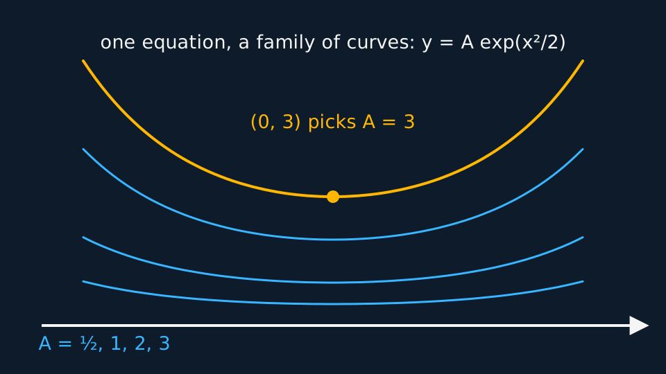
Write the single constant at the integration step, before any rearranging. Separating dy/dx = xy gives ln y = x2/2 + c, and exponentiating turns that constant into a multiplier, y = Aex²/2 with A = ec. Added afterwards, as y = ex²/2 + c, it gives a function that does not satisfy the equation.
Separate, integrate, solve
A separable equation has the form dy/dx = f(x)g(y). Solve g(y) = 0 first: each root k gives a constant solution y = k, which satisfies the equation but is lost on dividing by g(y). Then, where g(y) ≠ 0, divide by g(y) so that every term in y is on one side and every term in x on the other.
Both sides are then standard integrals, and a single constant c, written at the point of integration, covers both.
WORKED EXAMPLE
Separate, integrate, apply the condition
Solve dy/dx = xy for y > 0, given that y = 3 when x = 0.
Separate and integrate: ∫(1/y) dy = ∫x dx, so ln y = x2/2 + c.
Exponentiate: y = Aex²/2, where A = ec absorbs the constant. The question said y > 0, and that is what lets the modulus go and keeps A positive here.
The condition gives A = 3, so y = 3ex²/2.
Write the constant at the integration step. Adding it after exponentiating, as y = ex²/2 + c, gives a function that does not satisfy the original equation: exponentiating ln y = x2/2 + c turns the constant into the multiplier A = ec.
GUIDED PRACTICE
Factorise before separating
Solve dy/dx = xy + x, given that y = 1 when x = 0, before opening the working.
Show the working
The right side does not separate as written. Factorising fixes that: dy/dx = x(y + 1).
∫dy/(y + 1) = ∫x dx gives ln|y + 1| = x2/2 + c, so |y + 1| = ecex²/2.
Nothing here fixes the sign of y + 1, so the modulus comes off as a ±: y + 1 = Aex²/2 with A = ±ec, which is any non-zero constant. Taking A = ec alone would keep only y > −1 and lose the whole branch below it.
The condition gives A = 2, so y = 2ex²/2 − 1.
A = 0 is worth adding back. It returns y = −1, the constant solution that dividing by y + 1 threw away, and substituting it gives dy/dx = 0 and x(y + 1) = 0, so it does satisfy the equation. Allow every real A and y = Aex²/2 − 1 is the complete family: A > 0 above the line y = −1, A < 0 below it, A = 0 on it.
Factorising the right-hand side is what makes the equation separable. After that the method is as in the previous example, with two points to record: exponentiating ln|…| gives a constant of either sign, and A = 0 restores the constant solution.
Models with meaning
In context, a differential equation states how a modelled quantity changes, and its solution predicts the quantity over time. A complete answer interprets that solution: state its behaviour for large t, the interval of t on which it applies, and the assumption that fails outside that interval.
WORKED EXAMPLE
The dissolving mint
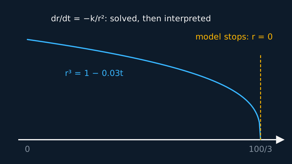
A spherical mint's radius decreases at a rate inversely proportional to the square of the radius: dr/dt = −k/r2, with r = 1 cm at t = 0. Solve for r.
Separate: ∫r2 dr = ∫−k dt, so r3/3 = −kt + c.
The condition gives c = 1/3, so r3 = 1 − 3kt.
With k = 0.01, r = 0 at t = 100/3 ≈ 33 minutes, and the model applies only for 0 ≤ t ≤ 100/3. The formula gives negative values of r beyond that, which no radius can take. State that interval as part of the answer.
INDEPENDENT PRACTICE
Slowing down
A particle moving in a straight line decelerates so that dv/dt = −0.2v, with v = 20 m s⁻¹ at t = 0. Find v(t), and comment on what the model says for large t.
Show the working
Separating, ∫dv/v = ∫−0.2 dt gives ln v = −0.2t + c, so v = Ae−0.2t with A = 20.
v = 20e−0.2t, halving roughly every 3.5 seconds.
For large t the model gives v approaching zero without reaching it. That behaviour follows from the modelling assumption: a resistance proportional to speed gives v = 0 only in the limit, whereas a constant frictional force brings the particle to rest in finite time. State that the long-term behaviour is a consequence of the assumption.
ASSESSMENT FOCUS
- Separate fully before integrating, factorising out any common factor first, and show the separated line as working.
- Write one + c at the integration step. A constant added after rearranging gives a function that does not satisfy the original equation.
- Exponentiating turns the constant into a multiplier, and that step should appear in the working. From ln|y| the multiplier is A = ±ec, any non-zero constant; a stated restriction such as y > 0 makes A = ec positive.
- A = 0 restores the constant solution removed by dividing by g(y). Include it when the question asks for the general solution.
- For a particular solution, substitute the condition into the general solution rather than into the differential equation.
- In context, state the interval on which the solution applies and its behaviour for large values of the variable.
CHECK YOURSELF
Solve dy/dx = y2 sin x, given y = 1 when x = 0, and state where the solution stops being valid.
Show a hint
∫y⁻² dy = ∫sin x dx, then the condition; watch the denominator.
Show the answer
Separating, −1/y = −cos x + c, and the condition y(0) = 1 gives c = 0.
So 1/y = cos x, that is y = 1/cos x.
y = 1/cos x is undefined where cos x = 0, so the solution through (0, 1) is defined on the maximal interval −π/2 < x < π/2 containing the initial point x = 0.
Separate the variables, integrate both sides, and write a single constant at the integration step; check g(y) = 0 first for constant solutions.
A particular solution comes from substituting the condition into the general solution, and in context it is valid only on an interval that must be stated.
WORKBOOK
Printable practice for this topic: original exam-style questions with room to work, and a fully worked answer book. Free to use; please do not redistribute or sell.
Or read them with their worked answers on the solving differential equations questions page.
USED LATER IN
CHECK YOUR PROGRESS
Rate how confident you feel with each objective for this lesson. Ratings are saved in this browser, on this device, unless you sign in.
- Solve first-order separable equations, factorising first where separation requires it, and retain the constant solutions lost by division.
- Turn a general solution into a particular one using a given condition.
- Interpret a solution in context, stating the interval on which it is valid and its behaviour for large values.
- Verify that a proposed solution satisfies the equation and its condition, by differentiating it and comparing both sides.
Open the full revision checklist to see every objective in the course in one place.